ABC and XYZ analysis in Excel with example of calculation
For the analysis of the assortment of goods, «prospects» of clients, suppliers, debtors are used methods ABC and XYZ (rarely).
Based ABC-analysis – is the famous Pareto principle, which states that 20% of efforts give 80% of the result. Transformed and detailed, this law has been applied in the development of we discussed methods.
ABC-analysis in Excel
ABC method allows you to sort a list of values in three groups, which have different impact on the final result.
- highlight the with the greatest "weight" in the total result;
- analyze the groups of positions instead of an extensive list;
- to work on one algorithm with the positions of one group.
The meanings in the list after the application of the method ABC are divided into three groups:
- A – the most important for the total of (20% gives 80% of the results).
- B – average in importance (30% - 15%).
- C - the least important (50% - 5%).
These values are not mandatory. Methods of determining the boundaries of the ABC-groups will differ in the analysis of various indicators. But if significant deviations are detected, you worth to think, what`s wrong.
Conditions for the using of ABC-analysis:
- the analyzed objects have numerical characteristic;
- the list of the analysis consists of homogeneous positions (you can not comparable washing machines and light bulbs, because these goods are occupied so different price ranges);
- were selected the maximum objective meaning (to rank the options on the monthly revenue more correct than on the daily receipts).
For some values, you can use the ABC analysis methodology:
- the commercial range of goods (analyzing to profit);
- the client base (analyzing to the volume of orders);
- the supplier base (analyzing to the shipments);
- the debtors (analyzing to the sum of indebtedness).
The ranking method is very simple. But to handle of large volumes of data without special programs is problematic. The tabular processor Excel greatly simplifies to the ABC-analysis.
The general scheme:
- Identify to the purpose of analysis. Determine the object (which analyze) and parameter (on what principle will be sorted by groups).
- Make the sorting parameters in descending order.
- Summarize to numeric data (parameters - revenue, the amount of debt, the volume of orders, etc.).
- Find the proportion of each parameter in the total.
- Calculate to the share of cumulative total for the each list value.
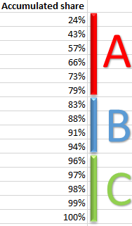
- Find the value in the list, in which the share of cumulative total is approaching to 80%. This is the lower limit of the group A. The top – is the first in the list.
- Find the value in the list, in which the share of cumulative total close to 95% (+ 15%). This is the lower limit of the group B.
- For C - everything below.
- Calculate the number of values for each category and the total number of positions in the list.
- Find the shares of each categories in total.
ABC-analysis of commercial range of goods in Excel
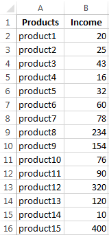
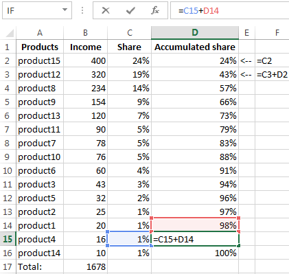
We form to the study table with 2 columns and 15 rows. We insert the names of the conditional goods and sales dates for the year (in the monetary value). It is necessary to rank the range of the income (which products provide more profit).
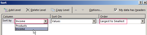
- Sort the dates in the table. Excrete to the entire range (except the top) and press «Sort» on the «Data» tab. In the dialog box has been opened, in the «Sort by» select «Income". In the column «Order» - «Largest to Smallest».
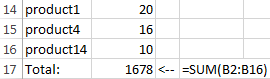
- Add in the table to the final line. We need to find the total sum of the values in the column «Income». Go to cell B17 and press the hotkey combination ALT + «=» for quick access to functions with filled parameters: =SUM(B2:B16).
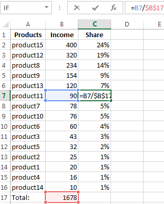
- To calculate the proportion of each element in the total amount. Create the third column «Share» and appoint for the cells to percentage format. Enter the formula in the first cell: =B2/$B$17 (the link to the "sum" we must do to the absolute). "Stretch" to the last cell of column. In addition, make «Percent» of cells format CTRL+SHIFT+5.
- Calculate the share by accrual basis. Add in the table the 4-th column «Accumulated share». For the first position, it will be equal to the individual share. For this purpose, the cell D2 enter: =C2. For the second position – is the individual share + share of accrual basis for the previous position. Enter in the second cell the formula: =C3+D2. "Stretch" until the end of the column. For the last positions it must be 100%.
- Assign by the positions to one or another group. Less than 80% - is in the group A. Less than 95% - is in the group B. Other ones – in the group S.
- To be comfortable to use the results of the analysis, affix in front of each item to corresponding letters.
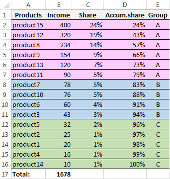
So we has been finished the ABC-analysis using Excel facilities. The further actions of the user – is the using of the findings dates in practice.
XYZ-analysis: the example of calculation in Excel
This method is often used in addition to the ABC analysis. The combined term ABC-XYZ-analysis is even found in the literature.
The acronym XYZ hides to the level of predictability of the predictability of the object being analyzed. This index is made to measure by the coefficient of variation that characterizes the measure of the scatter dates around the average value.
The coefficient of variation – is a relative measure, which does not have of the specific units of measurement. It`s suffice informative. Even per se. BUT! The tendency, seasonality dynamics significantly increase the rate predictability. As a result is reduced the rate predictability. This error may involve to wrong decisions. This is a huge minus of XYZ-method. It`s nevertheless…
There are possible objects for analysis: volume of sales, number of suppliers, revenue, etc. More often this method is used for determining the goods for which there is the strong demand.
XYZ-analysis algorithm:
- The calculation of the level of the coefficient of variation of demand for each product category. The analyst estimates the percentage deviation of the sales volume of the mean.
- Sort product range for the coefficient of variation.
- Position classification in the three groups - X, Y or Z.
The criteria for the classification and characteristic of the groups:
- «Х» - 0 - 10% (the coefficient of variation) - goods with the strongest demand.
- «Y» - 10 - 25% - goods with volatile sales.
- «Z» - 25% - goods having random demand.
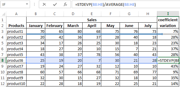
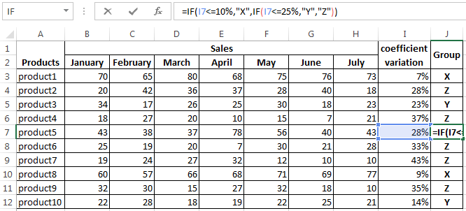
Compose the training table for XYZ-analysis.
- Calculate the coefficient of variation for each commodity group. The variability calculation formula of sales volume: =STDEVP(B8:H8)/AVERAGE(B8:H8).
- Classify meanings - define to the products in the group «X», «Y» or «Z». We use the built-in function «IF»: =IF(I3<=10%,"X",IF(I3<=25%,"Y","Z"))
Download ABC and XYZ analysis example in Excel
In the group «X» are got products that have the most stable demand. The average monthly sales volume rejects by only 7% (the product 1) and 9% (the product 8). If you have the stocks of these items in the stock, the company should put the products on the counter.
Stocks of goods from the group «Z» can be reduced. Or even go to these names on a pre order.
