Creating and managing tables in Excel

Creating a table in Excel may seem unusual at first. But it becomes clear that this is the best tool for solving this problem when you have mastered the first skills to work with this.

In fact Excel is a table consisting of a plurality of cells. All that is required from the user is to pick up table format for the subsequent work.



Let’s begin from next: highlight Excel cells you need using a mouse (holding the left button). After that you may choose formatting and apply it to the selected cells.

Following provisions will help to make a table in Excel as desired.

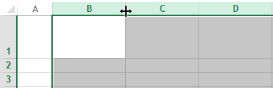
How to change the height and width of the selected cells? If you want to change cell sizes use fields with headers [A B C D] in horizontally way and [1 2 3 4] in vertically dimension. You have to move the cursor of a mouse on the border between the two cells. Holding down the left mouse button draw the border of the way and let it go.

In order not to waste time and may set the desired size to multiple cells or columns in Excel. To do this you have to activate the columns / rows by selecting them with the mouse on the gray field. It remains only to conduct already above described operation.

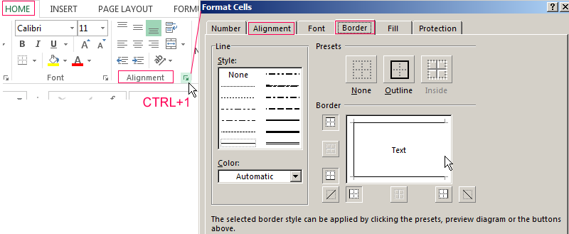
The window «Format Cells» can be caused by three simple ways:

1. The key combination Ctrl + 1 (the “1” is not on the numeric keypad, it’s above the letter "Q") is the fastest and most convenient way.
2. The context menu (right click).
3. Using the main menu «HOME» on the tab «Alignment».

Next, perform the following steps:

1. Click on the tab "Format Cells" hovering the mouse cursor
2. A window pops up with such tabs as «Number», «Alignment», «Font», «Border», «Fill» and «Protection».
3. You must use a tabs «Border» and «Alignment» to solve this task.

Tools in «Alignment» tab are the key capabilities for effective editing previously entered text in the cells, namely:

1. Merge the selected cells.
2. The ability to transfer the words.
3. Aligning the entered text vertically and horizontally (tab located in the top menu box as well as quick access).
4. Text orientation including vertical angle.

Excel makes it possible to carry out a rapid alignment of all previously typed text in vertical orientation using the tabs located in the Main Menu.

On the «Border» tab we are working with the lines style of table borders.



Flip the table: how to do it?

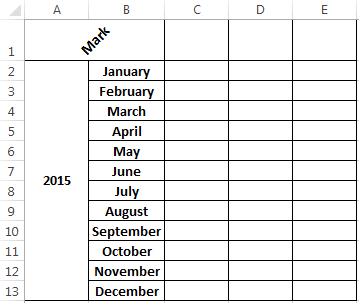
For example a user has created an Excel spreadsheet file of the following form:

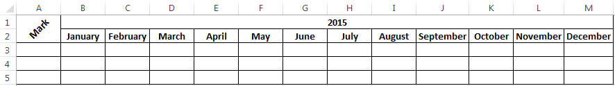
According to the task it is necessary to do so headlines in the table were positioned vertically and not horizontally as it is now. Proceed as follows.

First we need to highlight and copy the entire table. After that you must activate any empty cell in Excel. And then via the right mouse button displays a menu where you need to click the tab «Paste Special». Or you may press the key combination CTRL + ALT + V.

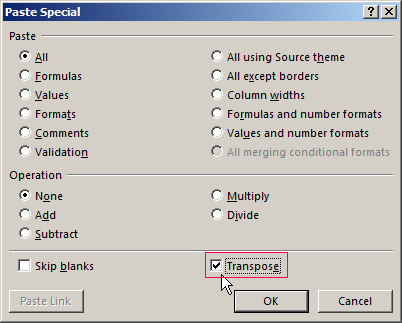
Next you need to establish a tick in the «Transpose» tab.

And press "OK" via the left button. As a result the user will receive:

Using transposition button you can easily transfer the values even in cases where a single table header stands vertically and in the other header stands horizontally.

How to transfer values from the vertical into the horizontal table

Many users are often faced with the seemingly impossible task - transferring values from one table to another, despite the fact that values are arranged horizontally in one table, and the other placed in the vertical way.

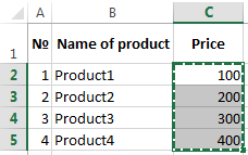
Assume that the user has an Excel price list which spelled out with the prices of the following form:

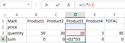
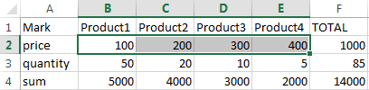
There is also a table where the total cost of the order is already calculated:

User task is to copy the values of the vertical price-list with prices and paste it into another horizontal table. It’s a long while and inconvenient to perform these actions manually by copying the value of each cell.

Use the tab «Paste Special» and transpose function in order to be able to copy all the values

Procedure:

1. The table with a price list and prices you must use the mouse to select all values. Then while holding the mouse over the previously selected field you must right-click and bring up a menu to select the "Copy":
2. Then selected range will be highlighted and you may paste previously allocated prices.
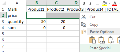
3. Using the right mouse button call menu and then, you must select the button «Paste Special» while holding the cursor over the selected area.
4. Finally set the check mark in «Transpose» button and press "OK".

As a result you get the following output:

Using the window «Transpose» you can completely turn the table. Function of transferring values from one table to another (taking into account their different locations) is a very handy tool. For example, it allows you to adjust the value quickly in the price list in case of the company's pricing policy has changed.

Changing the size of the table during the adjustment in Excel

It happens often when filled Excel table simply does not fit on the screen. And you have to move from side to side which is inconvenient and time consuming. You can simply change the table scale to solve this problem. it’s very comfortably to work changing scale if you have small or big display.

To reduce the size of the table go to the tab «VIEW» and select there the tab «Zoom». Then pick up an appropriate size for your screen. For example choose 80 or 95 percent. It also might be another scale.

To increase the size of the table use the same procedure with the slight difference that the scale is placed over one hundred percent. For example choose 115 or 125 percent.

Excel offers a wide range of possibilities for building fast and efficient work. For example using a special formula (for example, = OFFSET ($a$1;0;0счеттз($а:$а);2) you can adjust the dynamic range used by the table. That can be very convenient during work especially when you are working simultaneously with multiple tables.