Creating a database in Excel and its functionality
Any database (DB) is a summary table with the parameters and information. Most schools programs included the creation of a database in Microsoft Access. But Excel gives all the opportunities to build simple databases and easily navigate through them.
How to make the database in Excel so it was convenient not to only store but also process the data: generate reports, build charts, graphs, etc.
Step by step to create a database in Excel
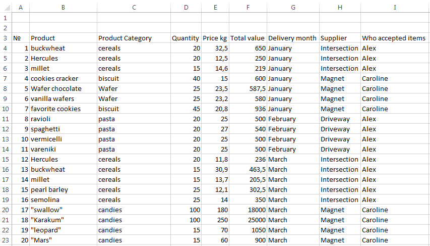
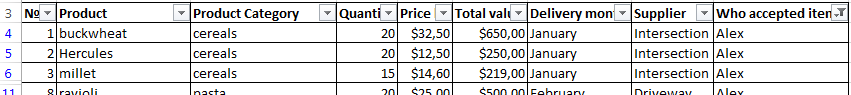
At first we will learn how to create a database using Excel tools. Let’s imagine that we are the shop. We draw up a summary table of data with various products deliveries from different suppliers.
| № | Product | Product Category | Quantity | Price kg | Total value | Delivery month | Supplier | Who accepted items |
We puzzled out with headlines. Now fill the table. We start with a serial number. We don’t have to put down the numbers manually. Enter in cells A4 and A5 one and two respectively. Then select those two cells with left mouse button and grab the corner of the segregation and extend down to any number of rows. In a small little window you will see the final number.
Note. This table can be downloaded at the end of the article.
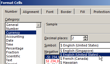
Base show us that some of the information will be presented in text form (product, category, month, etc.), and some is in the financial. Select the cells with the headlines named Price kg and Total value E4:F23. Use right-click to see context menu where choose «Format Cells» CTRL+1.
A window will appear where we will choose the Currency format. Enter the number of decimal places equals 1. We don’t have to choose designation because in the header we already pointed out that the price and value in $ English (United States).
Similarly we proceed with the cells where the quantity column will be filled. Select numerical number.
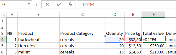
Let’s deal with another preparatory action. You can immediately use that fact that in the corresponding cells value is calculated as the price multiplied by the quantity. To make this we enter in cell F4 formula and stretch it to the other cells in this column. Thus the cost will be calculated automatically while filling the table.
Now fill the table with data.
It's important! It is necessary to stick to a single style of writing while filling the cells. If the original name of the employee is recorded as Alex AA, then the rest cells should be filled similarly. The work with the database will be difficult if somewhere name will be written differently, for example, Alexey Alex.
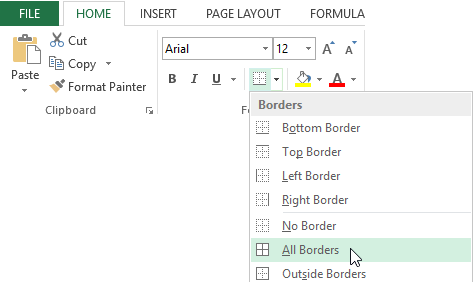
The table is ready. In reality it may be much longer. We have added a several positions for example. Let us give the database a more aesthetic appearance with making the frame. To do this select the entire table and find the parameter «All Borders» on the panel.
Similarly, frame the headlines thick outer boundary.
Excel functions for working with database
Now we turn to the functions that Excel offers to work with the database.
Working with databases in Excel
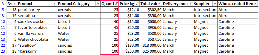
Example: we want to know all the products receipted by Alex AA Theoretically, you can run through the all rows visually where this name appears and then copy them to a separate table. But what if our database composed of several hundreds of items? FILTER comes to help us.
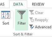
Select all the headlines in the table and click «FILTER» in the «DATA» tab, (CTRL + SHIFT + L).
In each cell in the header appears black arrow on a gray background which can be clicked to filter the data. Click it in the parameter WHO ACCEPTED ITEMS and remove the check mark from the CAROLINE name.
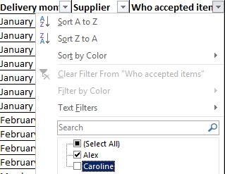
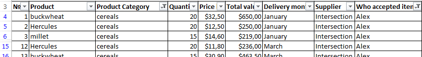
Thus there are remains data only with Alex.
Note! When you are sorting data not only all the positions in the columns stays in its places but rows of numbers also corresponding to the sheet (these are highlighted in blue). This feature is useful to us later.
You can make additional filtering. Determine which kind of grouts Alex accepted. Click the arrow on the cell PRODUCT CATEGORIY and leave only grouts.
If you need to return the full database you can make it in easiest way: set out all the checkboxes in the corresponding filters.
Data sorting
In this example the database was filled in chronological order during the supplying goods in the shop. But if we want to sort the data on a different principle excel allows you to do that too.
For example, we want to sort the products as price increase. Those the first line will be the cheapest product and in the last will be the most expensive. Select the column with the price and on the HOME tab and choose the «Sort & Filter».
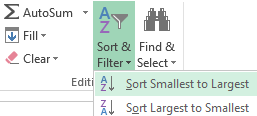
As we decided that lower price would be on top choose «Sort Smallest to Largest». You will see another window where we select «Expand the selection», so the other columns can also adjust to the sorting.
We see that the data is sorted in order to increasing price.
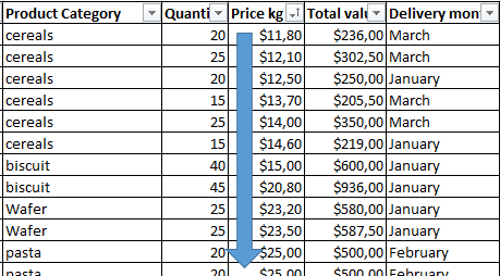
Note! You can make sorting in order to increase or decrease parameter using AutoFilter. Such action is also proposed when you press the arrow.
Sort by condition
We need to extract from the database products that were purchased in lots of 25 kg or more. For this purpose click the filter arrow on QUANTITY cell, and select the following options.
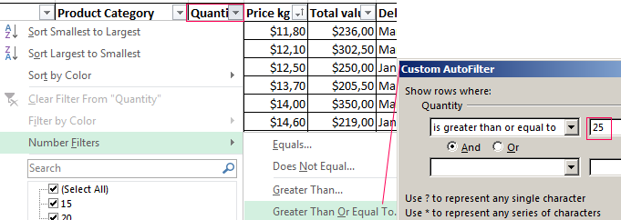
In the window that appears in front of condition БОЛЬШЕ ИЛИ РАВНО inscribe number 25. Then you will get sample indicating the products ordered by the lots greater than 25 kg or equal to this. Those products also sorted in the manner of its price growth since we did not remove sorting by price.
Subtotals
This is another useful function which allows calculating the sum, the multiplication, minimum or average value, etc. using the existing database. It is called the subtotals. =SUBTOTAL() This function has one main advantage. It allows making calculations with certain function even if you change the size of the table. Let’s consider it with an example.
Let us give our full database suitable view. Next we create a formula for the AutoSum in column Total value. Enter formula writing it in the F26 cell. At the same time remember how database sorting in Excel: number of rows fixed in place. Therefore the formula will still be in the F26 cell even when we do filtering.
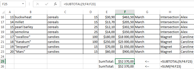
Subtotal function has 30 arguments. The first is static: the action code. By default Excel set code number 9, so let it be. The second and subsequent arguments are dynamic: this is links to ranges which are summed up. We have a range: F4: F24. It turned out 19,670 rubles.
Now try again to sort number, leaving only a party of 25 kg and >.
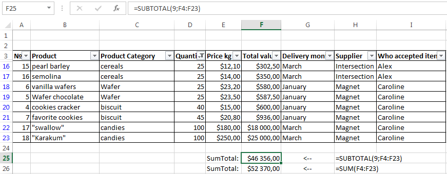
We see that the amount has changed, too.
In Excel, you can also create a small database and easy to work with them. When large volumes of data is very convenient and efficient.
