Download excel phone list template

Excel is useful for creating phone books. Moreover, the information is not just stored there securely, but it can also be used to perform various manipulations and comparison with other lists, etc.

So it’s very important to create phone list correctly to make it really a useful array.



Phone list template

How to make a phone list in Excel? It’s really easy! To create a phone list you need at least two columns: first column will consist of first names (or last names) of the person or organization and second one - of the phone numbers. But you can make the list more useful by adding additional rows.

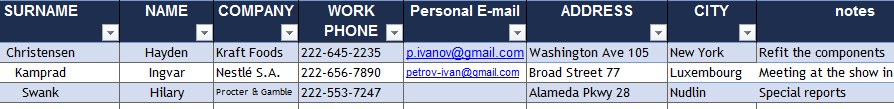
The columns header may be different, some columns may be added, some deleted. All you need is to fill out the list information.

Additionally, you can conduct another manipulation: to determine the cells' format. By default, the format of each cell is listed as «General». You can leave it as it is, but for a phone number column you can specify a custom format. To do this, select cells in this column, right-click to bring up the menu, choose «Format Cells».

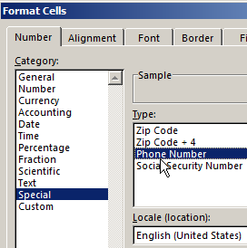
Among the given options select «Special». On the right you'll see a mini-list, in which you need to select «Phone Number».



How to use the phone list

Any data directory is needed for easy work with information, for example, by using a single criterion to know the rest. So, in the phone list, we can enter the required last name and get the phone number of this person. To do this in Excel there are functions «INDEX» and «MATCH».

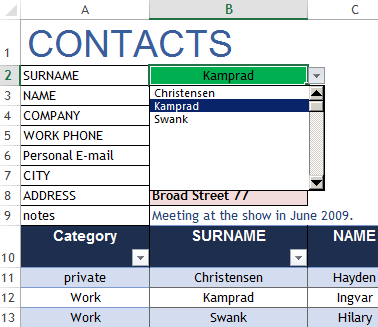
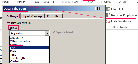
So, we have a little phone book. In reality, the firms usually have longer lists, so to look for information in them manually is very difficult. Let's make the preform, which will contain all the information. And it will appear on specific criteria - last name, therefore we will make this item in form of a dropdown list («DATA»– «Data Validation» – «Allow:» – «List»).

You need to do the following: by choosing some of the last names, all other cells have to be automatically stamped with the appropriate information. The cells with phone number have to be highlighted in green because it’s the most important information.

In cell J6 (where «NAME»), enter the command =INDEX and begin to fill up the arguments.

1. Array: select the whole table of orders together with a header. Make it absolute, by pressing F4.
2. Line number: here you enter «MATCH» and fill up the arguments of this function. The search value will be a cell with a dropdown list – J6 (plus F4). The column with last names (together with header) will be the overlooking array: A1:A13 (plus F4). Type of matching: exact match, i.e. 0.
3. Column number: and again you need to use «MATCH». The search value: I7. The array: the header of the array, i.e. A1:H1 (F4 plus). Type of matching: 0.

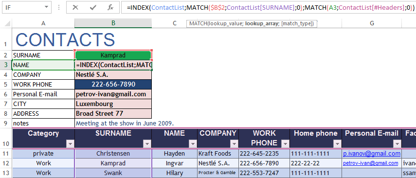
We have received the following. The formula is universal, it can be used for the remaining lines in the preform. Now, when choosing last names, all other information will be dropdown. Including a phone number.

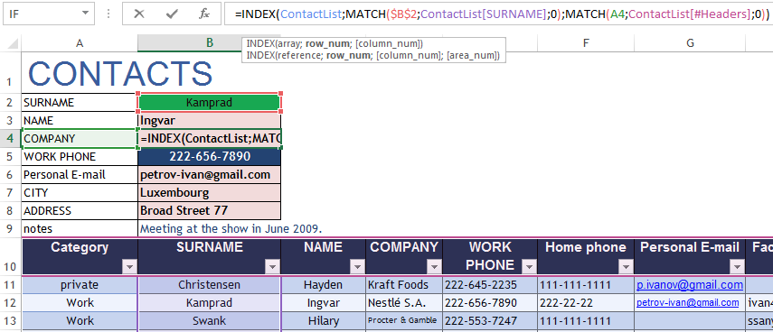
It turns out that the «INDEX» command, when you specify the criteria in the array, gives the number of its row and column. But since the criterion is non-constant, and we will constantly change the last name to find out phone numbers of people, we have additionally used the «MATCH» function. It helps to find the position of the desired row and column.

How to compare two lists in excel

Working with lists in Excel implies a comparison: comparing data, finding the same or unique items. Let's try for example to compare two simple lists.

There is information on the two warehouses. Our task: to check up, what positions are missing on both warehouses to make in the future the order and deliver the missing products.

Highlight both lists (without headers) using the CTRL key. We don't need the space between the lists (i.e. column B). Then on the «HOME» tab, select «Conditional Formatting» – «Highlight Cells Rules» – «Duplicate Values».

A small window will appear where you can choose to command showed duplicate or unique values. Choose «Unique». They will be highlighted in color that you can choose the list on right. We have it red.

Download Excel phone list template

Now you can copy all of the red cells from the left column and add them to right and vice versa. And now we get two equivalent lists.