COUNTIF function in Excel and examples of using it
The COUNTIF function is included in the group of statistical functions. It allows you to find the number of cells by a certain criterion. The COUNTIF function works with numeric and text values, as well as with dates.
Syntax and features of the function
First, let’s consider the arguments:
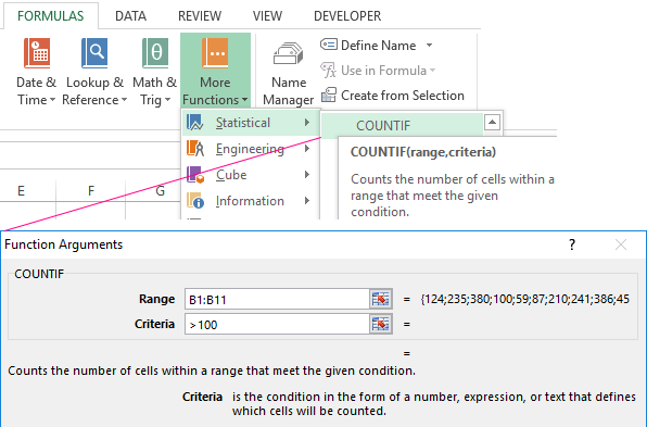
- Range – the group of values for analysis and counting (required).
- Criteria – the condition by which cells are to be counted (required).
The range of cells can include textual and numerical values, dates, arrays, and references to numbers. The function ignores empty cells.
A criterion can be a reference, a number, a text string, or an expression. The COUNTIF function only works with one criterion (by default). However, you can “force” it to analyze two criteria simultaneously.
Recommendations for the correct operation of the function:
- If the COUNTIF function refers to a range in another workbook, this workbook must be opened.
- The «Criteria» argument must be enclosed in quotation marks (except for references).
- The function does not take into account the letter case.
- When formulating a counting condition, you can use wildcard characters. The question mark "?" is any character. The asterisk "*" is any sequence of characters. For the formula to search for these signs directly, put a tilde (~) before them.
- For normal operation of the formula, cells with text values should not contain spaces or non-printable characters.
Countif function in Excel: examples
Let’s count the numerical values in one range. The counting condition is one criterion.
We have the following table:
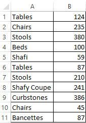
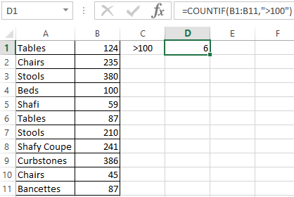
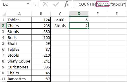
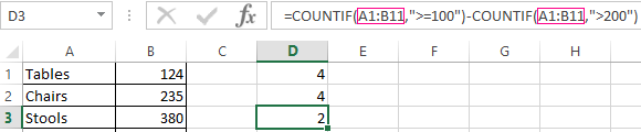
Count the number of cells with numbers greater than 100. Formula: =COUNTIF(B1:B11,">100"). The range is В1:В11. The counting criterion is ">100". The result:
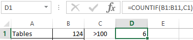
If the counting condition is entered in a separate cell, you can use the reference as a criterion:
Count the text values in one range. The search condition is one criterion. Formula: =COUNTIF(A1:A11,A3).
Or used reference inside the table:
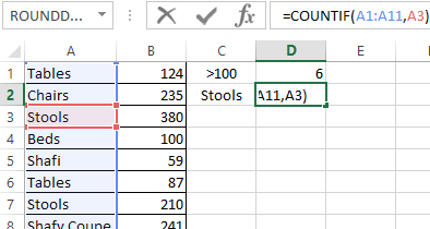
In the second case, the cell reference was used as a criterion, result is the same – 2.
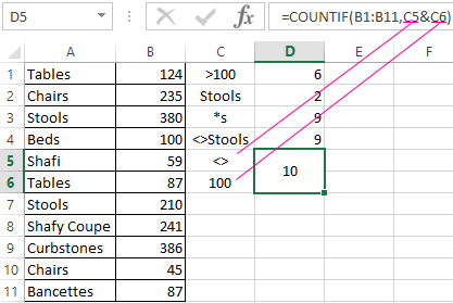
Formula with the wildcard character application: =COUNTIF(A1:A11,"Tab*"). To calculate the number of values ending in «и» and containing any number of characters: =COUNTIF(A1:A11,"*s"). We obtain:
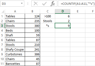
All names that end with a letter «s».
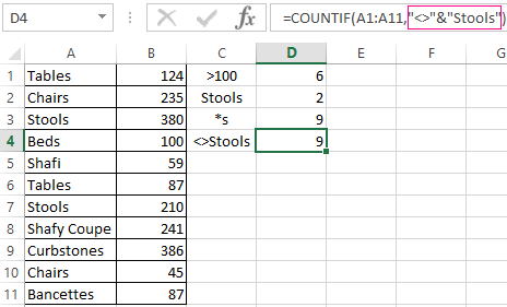
We use the search condition "not equal" in the COUNTIF.
Formula: =COUNTIF(A1:A11,"<>"&"Stools"). The operator "<>" means "not equal". The ampersand sign (&) is used to merge this operator and the “Stools” value.
When you apply a reference, the formula will look like this:
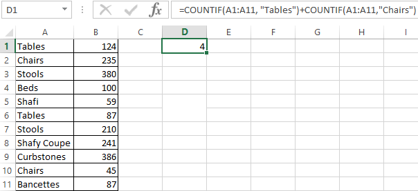
Often you need to perform the COUNTIF function in Excel by two criteria. In this way, you can significantly expand its capabilities. Let's consider special cases of using the COUNTIF function in Excel and examples with two criteria.
- Let's count how many cells are contained in the " Tables " and " Chairs " text. Formula: To specify several criteria, several COUNTIF phrases are used. They are united by the "+" operator.
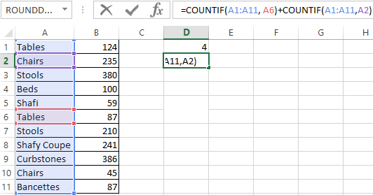
- Criteria – cell references. Formula: The function searches for " Tables " text in cell A1 and " Chairs " text – in cell A2 based on the criterion.
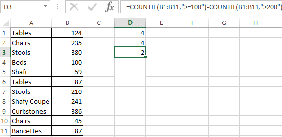
- Count the number of cells in B1:B11 range with a value greater than or equal to 100 and less than or equal to 200. Formula:
- Apply several ranges in the COUNTIF function. This is possible if the ranges are contiguous. It searches for values by two criteria in two columns simultaneously. If the ranges are not adjacent, then the COUNTIFS function is used.
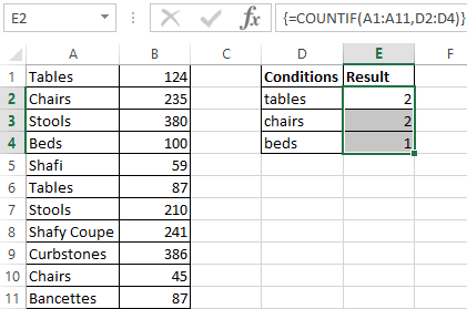
- When the criterion is a reference to a range of cells with conditions, the function returns the array. To enter a formula, you need to highlight as many cells as the range with criteria contains. After entering the arguments, simultaneously press Shift + Ctrl + Enter control key combination. Excel recognizes the formula of the array.
COUNTIF with two criteria in Excel is very often used for automated and efficient data handling. Therefore, an advanced user is highly recommended to carefully study all of the examples above.
Subtotal command and the countif function
Count the number of goods sold in groups.
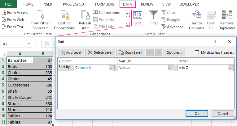
- First, sort the table so that the same values are close.
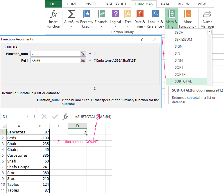
- The first argument of the formula “SUBTOTAL” – “Function number”. These are numbers from 1 to 11, indicating a statistical function for calculating the intermediate result. Counting the number of cells is carried out under number "2" (“COUNT”).
Download example COUNTIF in Excel
The formula has found the number of values for the «Chairs» group. For a large number of rows (more than a thousand), this combination of functions can be useful.
