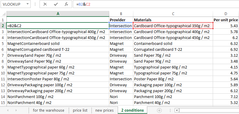
Function VLOOKUP in Excel for for beginners

The Function VLOOKUP in Excel allows rearranging data from one table to the corresponding cells in another one.

It’s very handy and frequently used. As it’s a problematic thing to compare manually ranges with tens of thousands of names.



How to use The Function VLOOKUP in Excel

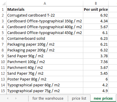
For example, the warehouse of the enterprise for the production of packaging received materials in a certain amount. The cost of materials is in the price list. This is a separate table.

It is necessary to find out the cost of materials received at the warehouse. To do this we should substitute the price of the second table in the first. And by ordinary multiplication we will find the title.

Algorithm:

1. Here is the first table (for the warehouse) in the required view. Add columns «Per unit price» and total «Price». Establish a currency format for the new cells.
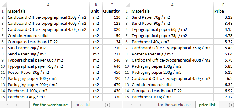
2. Select the first cell in the «Price» column. In our example it’s D2. Call the «Insert Function» using the «FX» button (at the beginning of the formula bar) or by pressing the hot key combination SHIFT + F3. In the category «Lookup & Reference» we find the function =VLOOKUP(), and click OK. This function can be called up by clicking on the «FORMULAS» tab and choose from the drop-down list of «Lookup & Reference».

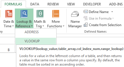
3. A window with the function arguments will be opened. In the field «Lookup_value» - the first column of the range of data from the table with the number of received materials. These are the values that Excel should find in the second table.
4. The next argument is «Table_array». This is our price list. Put the cursor in the field of argument than go to the list prices. Select the range with the names of materials and prices. Show what value the function should match.
5. For Excel to refer directly to these data, it is necessary to fix the link. Select «Table_array» field value and press F4. $ Icon appears.
6. In the argument «Col_index_num» put the number «2». Here are the data that you need to get in the first table. «Range_lookup» is FALSE. As we need specific, not approximate.

Click OK. And then copy the function of that column: we catch a mouse bottom right corner and drag down. We get the necessary result.

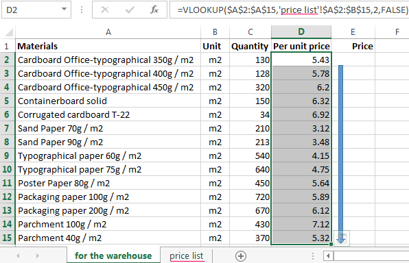
Now to find the cost of materials is not difficult: the number of * cost.

Function VLOOKUP linked the two tables. If you change the price, and then change the value of the materials received at the warehouse (now received). To avoid this, use the «Paste Special».

1. Select the column with inserted prices.
2. Use the right mouse button – «Copy».
3. Still selected use the right mouse button – «Paste Special».
4. Put a tick next to «Values». OK.

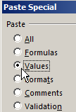
The formulas in the cells disappear. Only values remain.



A quick comparison of the two tables with the help of VLOOKUP

The function helps to compare the values in large tables. In case of the price has changed. We need to compare the old prices with the new prices.

1. In the old price list do the column «NEW Price».

2. Select the first cell and select the function VLOOKUP. The given examples (see. Above). For example:

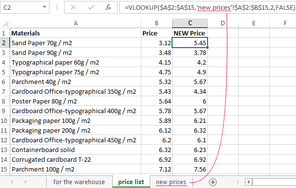
This means that you need to take the name of the material from the range A2: A15, look it up in the «new prices» in column A. Then take the data from the second column of the new price (Per unit price) and substitute them in cell C2 under «NEW Price».

The data presented in this way, can be compared. We can find the numeral and percentage difference.

The function VLOOKUP in Excel with multiple conditions

Until now, we have offered for the analysis of only one condition - the name of the material. In practice, it often requires several bands to compare and select the data value 2, 3 and other criteria.

Table for example:

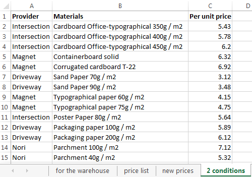
Guessing we need to find, what is the price of the corrugated cardboard of JSC «Magnet». It is necessary to set two conditions to search the name of the material and the vendor.

The matter is complicated by the fact that one supplier receives several names.

1. Adding to the table the leftmost column (important!), combining the «Provider» and «Materials».

2. We combine the required criteria the same way:
3. Put the cursor in the right place H3 and set arguments for function:

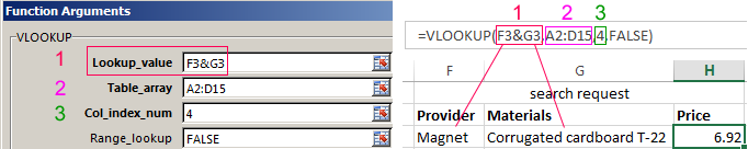
Excel finds the right price.

Consider the formula in detail:

1. What we are looking for – request the addition of a criterion F3&G3.
2. Where to look for – range of data A2:D15.
3. What data to take – column number 4 in the range A2:D15.

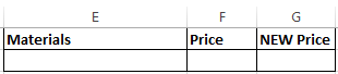
The Function VLOOKUP and drop-down list

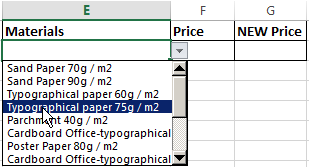
For example, some data is made in the form of a drop-down list. In our example it is «Materials». It is necessary to configure the function so that when choosing names appeared prices.

First do drop-down list:

1. Go to sheet «price list» and create a table for requests in the range E1:G2.

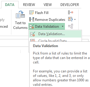
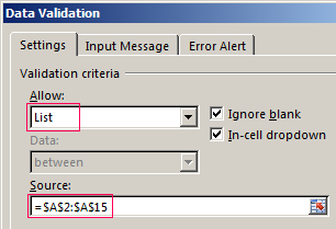
2. Put the cursor in cell F3, where will be this list and go to the tab «DATA». «Data Validation» menu.

3. Select the type of data – «List». Source is the range with the names of materials.

4. When press the OK the dropdown list is formed.

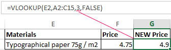
Now you need to make the way when choosing a particular material in the column price corresponding figure appeared. Put the cursor in the F2 cell (which will have to appear the price).

1. Open the window «Insert Function» and select VLOOKUP.
2. The first argument is «Lookup_value» – the box with drop-down list. The table is a range of materials with names and prices. And column 2. Function has acquired the following form:
3. In a cell G2, enter the formula (formula different column number 3):
4. Press ENTER and enjoy the result.

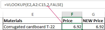
Change the material - the price changes:

Download this example VLOOKUP in Excel

This is how the drop down list in Excel with the function of the VLOOKUP. Everything happens automatically within a few seconds. Everything works quickly and accurately. It is necessary to deal with this function.