How to use the VLOOKUP function in two tables Excel
VLOOKUP in Excel is a very convenient and often used tool for working with tables, database and not only. This function is easy to learn and very functional in execution.
Due to a harmonious combination of simplicity and functionality of VLOOKUP, users actively use it in the process of working with spreadsheets. But it is worth noting that this function has many shortcomings that limit the possibilities. Therefore, it sometimes needs to be used with other functions or generally replaced with more complex ones. To begin with, let's consider its advantages on a ready-made example of a function and then determine the shortcomings.
How the VLOOKUP function works in Excel: an example
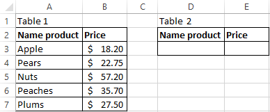
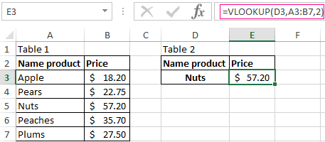
The VLOOKUP function is used to retrieve data from an Excel table using certain search criteria. For example, if the table consists of two columns: "Product name" and "Price". Nearby is another table, which will search in the first table using the criteria “name of the product” and get the value of the corresponding price.
- We move to the cell of the second table under the name of the column "Price".
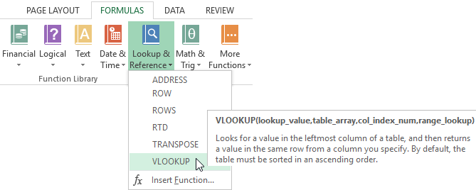
- Choose "FORMULAS" - "Lookup and Reference" - "VLOOKUP".
 You can also enter =VLOOKUP() using the "Insert Function". To do this, click on the "fx" button, which is at the beginning of the formula bar. Or you can press the hotkey combination SHIFT+F3.
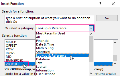 In the appeared dialog box on the category field, select the "Lookup and Reference" from the drop-down list, and then specify the function below.
 - We fill in the arguments of the function.
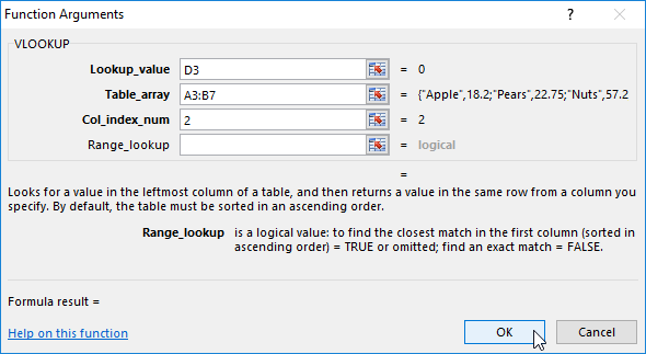
In the "Lookup_value" field, we enter a reference to the cell under the product name of the second table D3. In the "Table_array" field enter the range of all values of the first table A3: B7. In the "Col_index_num" field we enter the value "2", because in the second column we have the price that we want to receive when searching for the goods. And click OK.
Now enter the names of the goods for which we need to know its price under the column headline of the second table "Name product". And press Enter.
The function allows us to quickly find the data and get all the necessary values from the large tables. It's like working with databases. When a query is created to the database, the results are output which is a response to the query criteria.
The VLOOKUP function in Excel and the two tables
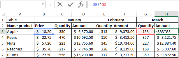
Let's slightly complicate the task changing the structure and increasing the amount of data in the table. Expand the amount of data in the first table by adding columns: "January", "February", "March". There we will record the sales amounts in the first quarter as shown in the picture:
As you can see, the second table also needs to be changed a little, so as not to lose the essence of the task.
Now we need to make a selection of data using the VLOOKUP function separately for the product and sum up the sales for the first quarter. To do this go to cell H3 and fill in its arguments as follows after calling the function:
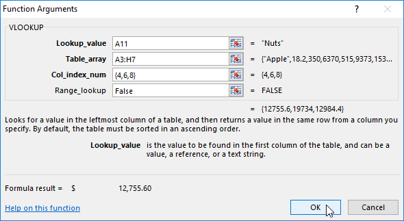
- Lookup value: A11.
- Table array: A3: H7. The range of our table is extended.
- Column index number: {4,6,8}. We need to use the function to simultaneously address several columns, so the value of this argument will be taken into the array by curly braces. And column numbers should be listed through a semicolon.
- Range lookup: FALSE.
- Then the entire function must be placed inside the SUM () function for the values in the selected columns to be summed. The whole formula is as follows:
- After entering this formula, you should press the key combination: CTRL+SHIFT+ENTER. Note! If you do not press a combination of these keys, the formula will work erroneously. In Excel, sometimes you have to perform functions in an array. You must use the keys CTRL+SHIFT+ENTER when entering formula. Then in the formula line, all the content will be taken in curly brackets "{}", which indicates the execution of the formula in the array.
Now enter the name of the product in cell A11 and in cell B11 we get the sales amount in the first quarter for this product.
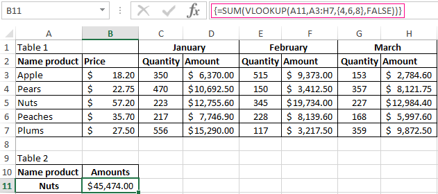
Comparison of two tables in Excel is performed by the VLOOKUP function and as soon as the matching of the requested data is determined, their values are immediately substituted for summation by the SUM function. The entire process is performed cyclically thanks to an array of functions as indicated by the curly brackets in the formula bar.
Note. If you enter the curly braces manually in the formula string, this will not work. You can execute the formula with a cyclic array only through a combination of hot keys: CTRL+SHIFT+ENTER.
Download example VLOOKUP function in two tables
It is worth noting that the main disadvantage of the VLOOKUP function is the inability to select several identical initial values in the query. In other words, if in our table the values "pear" and "apple" are repeated, we cannot sum up all the pears and apples. To do this, use the LOOKUP () function. It is very similar to the VLOOKUP but it is able to work well with arrays in the initial values.
