Transferring of table data via the VLOOKUP function
VLOOKUP in Excel is a very useful function, that allows you to pull data from one table to another one according by the given criteria. This is the fairly «smart» command, because the principle of its work consists of several actions: scanning of the selected array, selecting of the desired cell and transferring data from it.
The entire process of viewing and retrieving data occurs in fractions of a second, so we get the result immediately.
VLOOKUP Syntax function
VLOOKUP stands for vertical viewing – that is, the command transfers data from one column to another one. For work with the lines, there is a horizontal view – HLR.
The arguments of the function are as follows:
- the sought value is that is expected to be searched in the table;
- the table – there is the array of data from which the data are pulled. Notably, that the table with the data should be to the right of the original table, otherwise the functions of the VLOOKUP will not work;
- the column number of the table from which the values will be pulled;
- the interval review – there is the logical argument, that determines the accuracy or approximation of the value (0 or 1).
How do I move data using VLOOKUP?
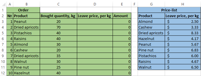
Let's consider the example in practice. We have the table in which the consignments of ordered goods are registered (it is highlighted in green). There is the price on the right, where the prices of each product are indicated (highlighted in blue). We need to transfer the price data from the right table to the left one to calculate the cost of each batch. Manually to do this for a long time, so use the Vertical Scan function.
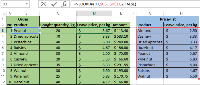
In the cell D3 you need to pull up to the price of peanut from the right table. Write = VLOOKUP and fill in the arguments.
The required value is the peanut from the cell B3. It is important to put the cell number, not the word «peanut», so then you can stretch to the formula down and get the remaining valuesautomatically.
The table – to select the price without the cap. That is to say, the names of the goods and prices. We fix this array with the F4 key, so that it does not change whenthe formula is drawn.
The column number – this is the number 2 in our case, because the necessary data (price) is in the second column of the selected table (price).
The interval review – we set 0,because we need to exact values, not approximate ones.
We see, that the price of peanut has risen from the right table to the left one.
Formula:
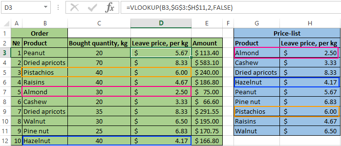
We pull up to the formula down and visually check some products to understand, that everything was done correctly.
Download example transferring of table via VLOOKUP function
Like so, with the helping of elementary actions, you can substitute to values from one table to another one. It is important to remember, that the Vertical View function works only if the table from which the data is pulled is on the right. Otherwise, you need to move it or use the INDEX and MATCH command. Having mastered these two functions, you will be able to realize more complex solutions much more than those provided by the VLOOKUP or HLOOKUP function.
