Examples of using SUMIF function with some criteria in Excel
Probably everyone can summarize data in Excel program. But with the improved version of the SUM function, which is called SUMIF, the capabilities of this operation are significantly expanded.
By the name of the function, you can understand that it does not only calculate the sum, but also complies with some logical conditions.
SUMIF and its syntax
The SUMIF function allows you to sum cells that meet a certain criterion (a given condition). The arguments of the function are as follows:
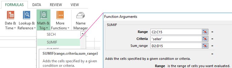
- Range - cells, which should be evaluated on the basis of the criterion (the specified condition).
- Criteria, determining which cells from the range will be selected (written in quotation marks).
- Sum range - the actual cells that are needed to be summed if they meet the criterion.
Consequently the function has only 3 arguments. However, sometimes the third one can be excluded, and then the command will work only by the range and criteria.
How does the SUMIF function work in Excel?
Let's consider the simplest example, which will clearly demonstrate how to use the SUMIF function and how convenient it can be for solving certain tasks.
We have a table in which the names of employees, their gender and salary, calculated for January are indicated. If we just need to calculate the total amount of money that is required to pay out to employees, we use the SUM function, specifying all salaries by the range.
But what do we have to do if we need to quickly calculate only sellers’ salaries? In this case, the use of the SUMIF function will help.
Enter the arguments.
- The range in this case will be a list of all staff posts, because we will need to determine the whole amount of salaries. Therefore, enter E2:E14.
- The criterion of choice in our case is the seller. Enclose the word in quotation marks and put it as the second argument.
- The range of summation is salaries, because we need to know the amount of salaries of all sellers. Therefore, enter F2:F14.
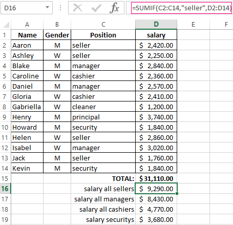
We have obtained 9290$. It means that the function automatically elaborated the list of all posts, chose only sellers from them and summed up their salaries.
Similarly, you can calculate the salaries of all managers, vendors, cashiers and security guards. When the table is small, it seems that everything can be counted manually, but when working with lists having several hundreds of positions, it makes sense to use SUMIF function.
SUMIF function in Excel with multiple criteria SUMIFS
If the letter S is added to the end of the standard SUMIF command, then it implies the function with several criteria (SUMIFS function). It is used in the case when you need to specify more than one criterion.
Syntax of using the function by several criteria
There can be as many arguments for SUMIFS as you like, but no less than 5.
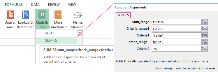
- Sum range. If in SUMIF it was at the end, then here it is in the first place. It also indicates the cells that need to be summed.
- Criteria range 1 - cells that need to be evaluated on the basis of the first criterion.
- Criteria 1 - defines the cells that the function will select from the first range of the condition.
- Criteria range 2 - cells, which should be evaluated on the basis of the second criterion.
- Criteria 2 - defines the cells that the function will select from the second condition range.
And so on. Depending on the number of criteria, the number of arguments can increase in an arithmetic progression in step 2. That is, 5, 7, 9 ...
Example of use
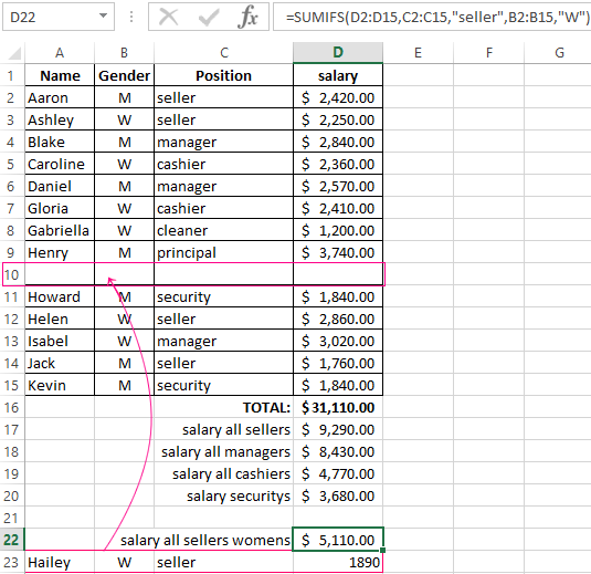
Suppose we need to calculate the amount of salaries of all female sellers for January. We have two conditions. The employee must be:
- a seller;
- a woman.
So, we will use the SUMIFS command.
Enter the arguments.
- Sum range - cells with a salary;
- Criteria range 1 - cells indicating the post of the employee;
- Criteria 1 - the seller;
- Criteria range 2 - cells with gender of the employee;
- Criteria 2 - female (f).
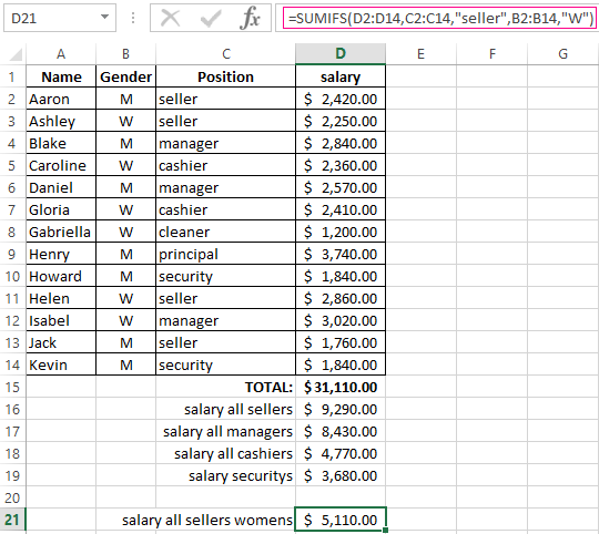
The result: all female sellers in January received in summation 5110$.
SUMIF in Excel with dynamic criterion
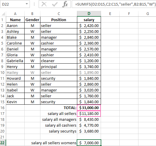
The SUMIF and SUMIFS functions are useful because they automatically fit themselves to the changing criteria. That is, we can change the data in cells, and the sums will change with them. For example, when calculating salaries, it turned out that we forgot to take into account one employee who works as a seller. We can add one more line by right-clicking and selecting the ВСТАВИТЬ command.
We have an additional row. We can see that the range of conditions and summations has automatically expanded to 15 rows.
Copy the employee's data and paste it into the general list. The sums in the resulting cells have changed. The functions have reacted to the appearance of another female seller in the range.
Similarly, you can not only add, but also delete any rows (for example, when the employee is discharged), change the values, etc.
