Conditional formatting training in Excel with examples

Conditional formatting is a convenient tool for data analysis and visual representation of results. Knowing how to use this tool will save you a lot of time and effort. A fleet glance at the document will be enough to obtain the necessary information.

How to apply conditional formatting in Excel

The tool «HOME»-«Conditional formatting» can be found on the main tab in the «Styles» section. If you click on the little arrow on the right, it will open the menu.

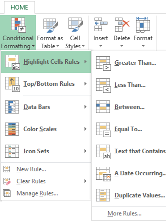
Let's compare the numerical values in an Excel range with a numerical constant. The rules «Greater Than / Less Than / Equal To / Between…» are the most frequently used. That's why they're listed in the menu «Highlight Cells Rules».

Let's enter some numbers in the range А1:А11.

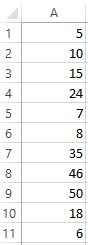
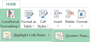
Select the range of values. Open the menu «Conditional formatting». Select «Highlight Cells Rules». Set a condition, for example, «Greater Than».

Let's enter the number 15 in the left box. In the drop-down menu on the right select the way of highlighting the values that correspond to the established condition: «Format cells that are GREATER THAN:» 15. The result is plain to see immediately:

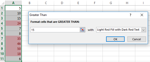
Leave this menu by hitting the OK button.

Conditional formatting by a cell's value

Let's compare the values in the range А1:А11 with the number in the B2 cell. Enter the number 20 in it.

Select the initial range and open the window of the «Conditional formatting» tool. In this example, let's apply the condition «less» («Highlight Cells Rules» - «Less Than»).

In the left box, enter the link to the B2 cell (click on this cell and its name will appear in the box automatically). The link's absolute by default.

The formatting result is plain to see in the Excel sheet immediately.

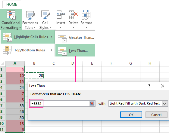
The values in the А1:А11 range that are less than the value of the B2 cell are filled with the selected color.

Let's set the following formatting conditions: compare the values of cells in different ranges and highlight the same values. We will compare the column А1:А11 with the column В1:В11.

Select the initial range (А1:А11). Click «Conditional formatting» - «Highlight Cells Rules» - «Equal To». In the left box, enter the link to the B1 cell. The link should be Mixed or Relative! And not absolute!

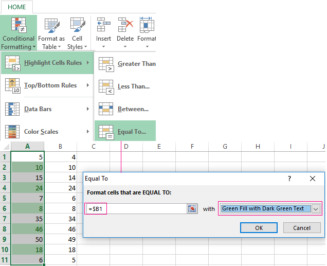
The program has compared every value in the A column with the corresponding value in the B column. The coinciding values have been highlighted with a fill color.

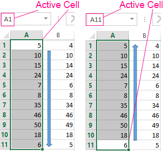
Important note! When you use relative references, you have to pay attention to which cell was active the moment you opened the «Conditional formatting» tool. Since it's the active cell to which the reference in the condition is “tied.”

In our example, the A1 cell was active at the moment we opened the tool. The link is $B1. Consequently, Excel compares the value in the A1 cell with the B1 value. If we selected the column from the bottom upwards rather than from top to bottom, the A11 cell would be the active one. And the program would compare B1 with A11.

Compare:

Pay attention to this nuance in order to ensure the «Conditional formatting» tool performs the task properly.

You can do the following to check the accuracy of the established condition:

Select the first cell in the range to which conditional formatting is applied.
Open the tool's menu; click «Manage Rules».

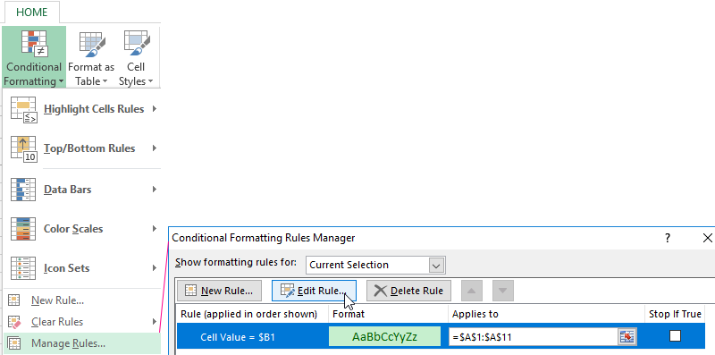
In the newly-opened window, you can see which rule is applied to which range.

Conditional formatting – several conditions

The initial range is А1:А11. We need the numbers that are greater than 6 to be highlighted with red. Green for numbers greater than 10. Yellow for values greater than 20.

Method: Select the range А1:А11. Apply «Conditional formatting» to it. «Highlight Cells Rules» - «Greater Than». Enter the number 6 in the left box. In the right one, select «Light Red Fill Dark Red Text». Hit OK. Select the range А1:А11 once again. Set the formatting condition as «Format cells that are GREATER THAN:» 10, and choose «Green Fill Dark Green Text». In the same way, set the yellow fill color for numbers greater than 20.

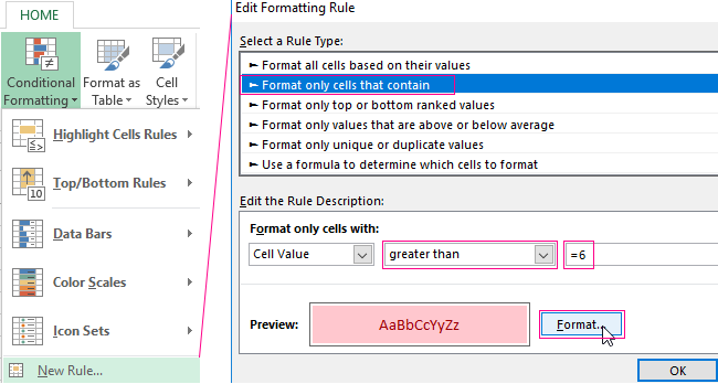
Method: Go to the menu of the «Conditional formatting» tool and select «New Rule». Fill in the formatting parameters for the first condition. Click OK. Likewise, set the second and third formatting conditions:

Note: the values in some cells simultaneously corresponds to two or more conditions. The highlighting priorities depend on the order of the rules listed in «Rules Manager».

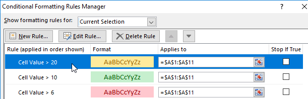
That is, the number 24, which is simultaneously greater than 6, 10, and 20, is highlighted in accordance with the condition «=$А1>20» (the first one on the list).

Conditional formatting of dates in Excel

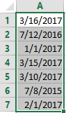
Select the range containing the dates.

Apply «Highlight Cells Rules»-«A Date Occurring» to it.

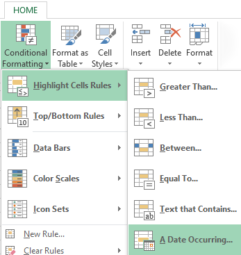
In the newly-opened window, you can seen the list of available conditions (rules):

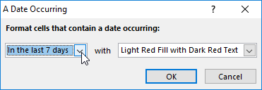
Select the suitable one (for instance, for the last 7 days) and click OK.

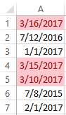
The red fill color highlights the cells containing the dates within the past week (the date when this article was written is March 3, 2017).

Conditional formatting in Excel using formulas

If the standard rules are not sufficient for the task, the user can apply a formula. The capabilities of this instrument are limitless, so virtually any formula can be used. Let's view a simple variant.

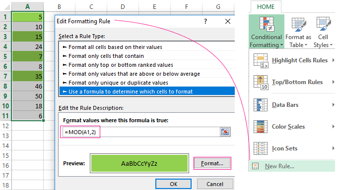
We have a column containing numbers. We need the cells with even numbers to be highlighted with a color. We will use the formula: =MOD(A1,2)

Select the range containing the numbers and open the «Highlight Cells Rules» menu. Select «New Rules». Click «Use a formula to determine which cells to format». Fill in the box as follows:

Click Ok to close the window and view the result.

Conditional formatting of the row by a cell's value

The task is to highlight the row containing a cell with a certain value.

The exemplary table:

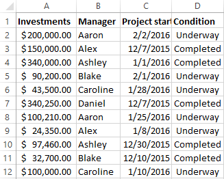
We need to highlight in red the information on the projects in progress («Underway»). For the completed projects' data («Completed»), the green fill in color should be applied.

Select the range containing the table values A2:D12. Click «Highlight Cells Rules»-«New Rule». Choose a formula as the type of condition. We will use the function: =IF().

The order of filling in the formatting conditions for «Completed projects».

Underway:

Completed:

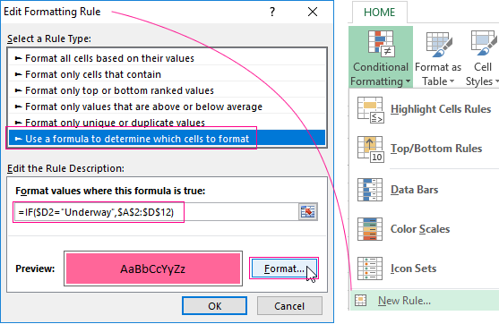
Note: links to a row are absolute; links to a cell are mixed (only the column is fixed).

Likewise, set the formatting rules for the projects in progress.

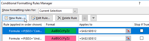
In «Rules Manager», the conditions appear as follows:

The obtained result:

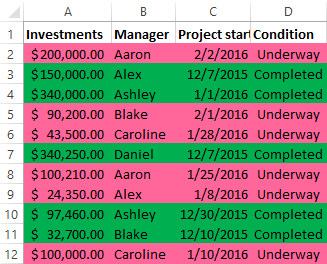
When the formatting parameters are set for the entire range, the condition will be fulfilled as soon as the cells are filled in. For example, let's complete Caroline project dated January 28 by replacing «Underway» with «Completed».

The highlight has changed automatically. It would have taken you a while to achieve this result using the standard Excel tools.