Conversion of the number in the currency format on the condition
For example the certain dataset contains in the table of transactions in EUR currency. We need to reformat automatically in the appropriate format to the value of column «Result». In Excel this task is easily solved by the conditional formatting.
How to convert the number in a money format by condition?
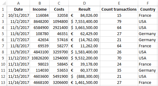
The table transaction of settlements with different countries in Euro currency:
The data in the «Result» column will be formatted in this way:
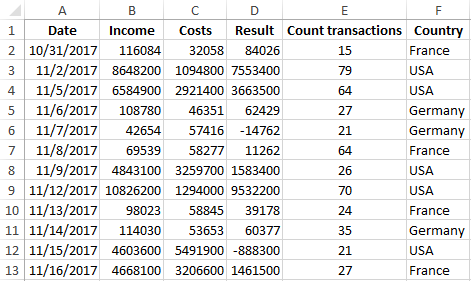
- if it the amount of USA – so the result is in dollars;
- if it the amount of any country from the EU – the result is in Euro-currency.
Let`s create the new rule with the formula:
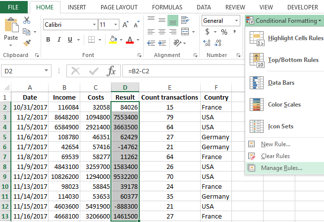
- Highlight to the cell range D2:D13 and select to the tool: «HOME» - «Styles» - «Conditional formatting» - «Manage Rules».
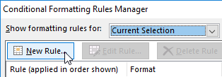
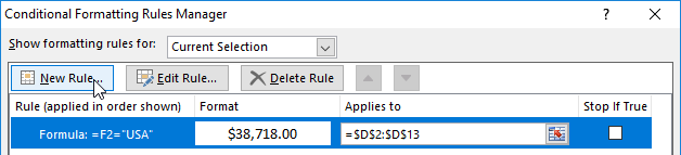
- In the new window «Conditional Formatting Rules Manager» click on the button «New Rule».
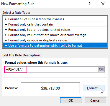
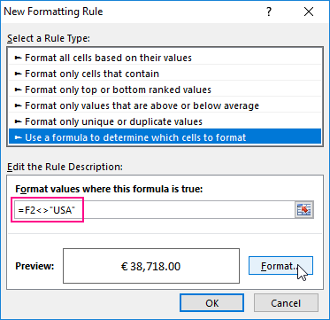
- Select: in window «New Formatting Rule» select the option «Use a formula to determine the which cells to format». And in the input box enter the formula: =F2="USA".
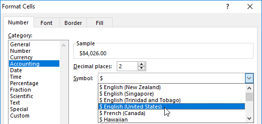
- Click on «Format» button and in the new window «Format Cells» in the tab «Number» select the appropriate currency as shown in the picture.
- After clicking on the windows «Format Cells» and «New Formatting Rule», you need to press OK and go back to the window Manager.
- There's also create the second rule. To do this, click on the appropriate button, and enter the formula: =F2<>"USA"
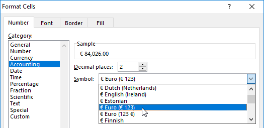
- Click on the button «Format» and in the window that appears «Format Cells», on the tab «Number» select to the specify currency of EUR.
- On all open windows to click «OK».
In the column D has been automatically formatted the numeric values in the appropriate monetary currency. Relativity of column F.
How to highlight with color to duplicate values in excel?
The exposure by color of the duplicates is one of the most popular tasks, in which is very handy to utilize the conditional formatting. For solving this, at first glance, complicated task it will be enough to make just a few clicks by mouse.
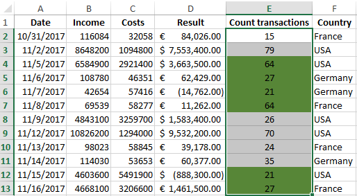
For example you need to find to the same number of transactions in the column E of the source table. For this purpose:
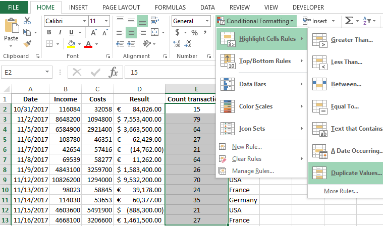
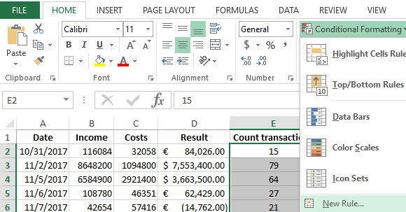
- To highlight the cell range E2:E13 and choose the tool: «HOME» - «Styles» - «Conditional formatting» - «Highlight Cells Rules» - «Duplicate Values».
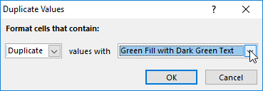
- In the new window from the left drop-down list to choose «Duplicate» and from the right one «Green Fill with Dark Green Text».
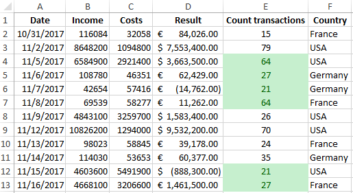
As a result, the cells with the same numbers of transactions are allocated by color.
For solution of the most tasks Excel provides to the several solutions. For example, to highlight duplicate values with color you can still in this way:
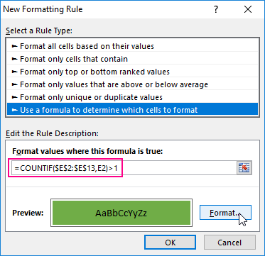
- When the selection E2:E13, you need to click the tool: «HOME» -«Styles» - «Conditional formatting» - «New Rule».
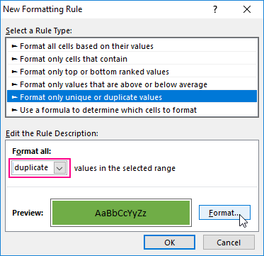
- In the new window «New Formatting Rule» at this time, to choose «Format only unique or duplicate values».
- The drop-down list «Format all:» must have the value «duplicate».
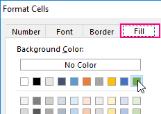
- Click on the button «Format» for setting to the green color on the tab «Fill». And click OK on all open windows of the program.
The more detailed analysis of using the formulas for finding duplicates is: how to find the same values in Excel column?
For searching duplicates, it is also possible to perform conditional formatting using the formula:
Download example conversion of number in currency.
But the first method is the easiest.
