How to hide or display rows and columns in Excel
Working in Excel, sometimes there is a need to hide part of displayed data.
The most handy way - is to hide individual columns or rows. For example, during the presentation or before preparing document to print.
How to hide columns and rows in Excel?
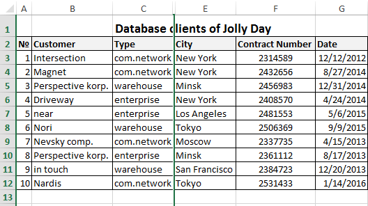
Let's say you have the table in what you need to display only the most significant data for better reading of performance. In order to do this, we will do the following:
- Select the column data of what you need to hide – for instance, the column C.
- On a selected column to right-click of mouse and select the option «Hide» CTRL+0 (for columns) CTRL+9 (for rows).
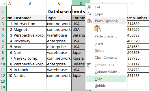
The column was hidden, but not deleted. This is evidenced by the priority of the alphabet`s letters in the names of columns (A; B; D; E).
Remark. If you want to hide multiple columns, highlight them before hiding. You can selectively highlight multiple columns with CTRL key pressed. In a similar way, you can hide the rows.
How to display hidden columns and rows in Excel?
To redisplay to the hidden column, you must select 2 of its contiguous (contiguous) columns. Then to generate the context menu, right-click and choose the option «Unhide».
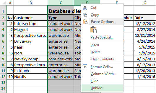
The similar actions are performed in order to open the hidden rows in Excel.
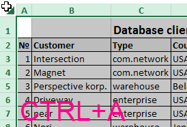
If the sheet is hidden many rows and columns and you want to display all at once, you must highlight the whole worksheet by pressing CTRL+A. Further a separate call to the context menu for the columns to choose the option «Show» and then for the rows, or in reverse order (for rows then for columns).
To select the entire sheet you can by clicking in the intersection of column headings and rows.
About these and other methods to select of an entire sheet and bands you have already known from the previous lessons.
