How to make a selection in Excel from the list with conditional formatting?
If you work with a large table and you need to search for unique values in Excel that corresponding to a specific request, then you need to use the filter. But sometimes we need to select all the lines that contain to certain values in relation to other lines. In this case, you should use the conditional formatting, which refers to the values of the cells with the query. To get the most effective result, we will use the drop-down list as a query. This is very convenient if you need to frequently change the same type of query to expose of the different table`s rows. We`ll look detailed below: how to make the selection of duplicate cells from the drop-down list.
Selection of the unique and duplicate values in Excel
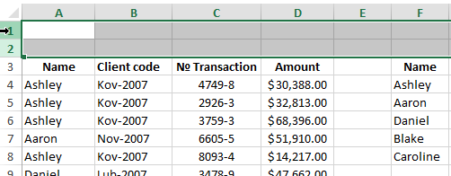
For example, we take the history of mutual settlements with counterparties, as shown in the picture:
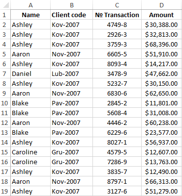
In this table, we need to highlight in color to all transactions for a particular customer. To switch between clients, we will use the drop-down list. Therefore, in the first place, you need to prepare the content for the drop-down list. We need all the customer names from the column A, without repetitions.
Before selecting to the unique values in Excel, we need to prepare the data for the drop-down list:
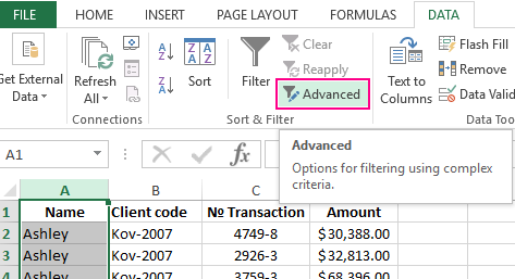
- Select to the first column of the table A1:A19.
- Select to the tool: «DATA»-«Sort and Filter»-«Advanced».
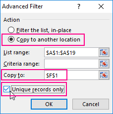
- In the «Advanced Filter» window that appears, you need to turn on «Copy the result to another location», and in the field «Place the result in the range:» to specify $F$1.
- Tick by the check mark to the item «Unique records only» and click OK.
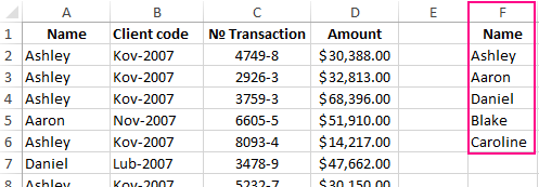
As a result, we got the list of the data with unique values (names without repetitions).
Now we need to slightly modify to our original table. To scroll the first 2 lines and select to the tool: «HOME»-«Cells»-«Insert» or to press the combination of the hot keys CTRL + SHIFT + =.
We have added 2 blank lines. Now we enter in the cell A1 to the value «Client:».
It's time for creating to the drop-down list, from which we will select customer`s names as the query.
Before you select to the unique values from the list, you need to do the following:
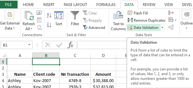
- In the cell B1 you need to select the «DATA»-«Data tool»-«Data Validation».
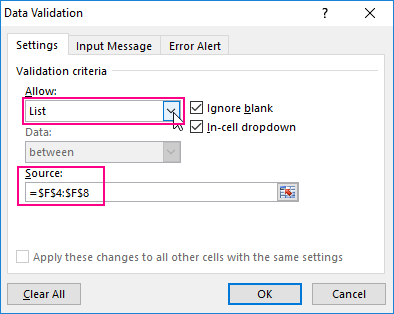
- On the «Settings» tab in the «Validation criteria» section, from the drop-down list «Allow:», you need to select «List» value.
- In the «Source:» entry field, to put =$F$4:$F$8 and click OK.
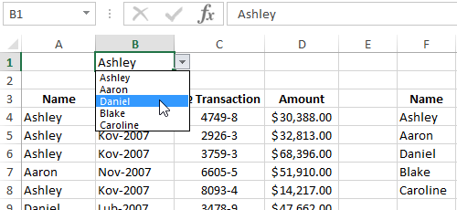
As a result, in the cell B1 we have created the drop-down list of customers` names.
Note. If the data for the drop-down list is in another sheet, then it is better to assign a name for this range and specify it in the «Source:» field. In this case this is not necessary, because all of these data is on the same worksheet.
The selection of the cells from the table by condition in Excel:
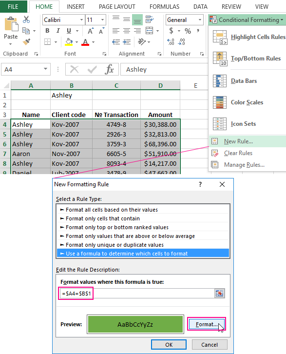
- Highlight the tabular part of the original settlement table A4:D21 and select the tool: «HOME»-«Styles»-«Conditional Formatting»-«New Rule»-«Use the formula to define of the formatted cells».
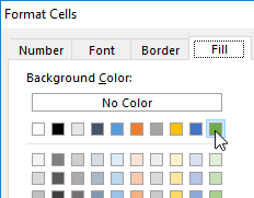
- To select unique values from the column you need to enter the formula: =$A4=$B$1 in the input field and click on the «Format» button to highlight the same cells by color. For example, it will be green color. And to click OK in all are opened windows.
It is done!
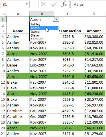
How does work the selection of unique Excel values? When choosing of any value (a name) from the drop-down list B1, all rows that contain this value (name) are highlighted by color in the table. To make sure of this, in the drop-down list B1 you need to choose to a different name. After that, other lines will be automatically highlighted by color. Such table is easy to read and analyze now.
Download example selection from list with conditional formatting.
The principle of automatic highlighting of lines by the query criterion is very simple. Each value in the column A is compared with the value in cell B1. This allows you to find unique values in the Excel table. If the data is the same, then the formula returns to the meaning TRUE and for the whole line is automatically assigned to the new format. In order for the format to be assigned to the entire line, and not just for the cell in column A, we use the mixed reference in the formula =$A4.
