What is the use of Pivot Table and Pivot Chart in Excel
The Pivot Table is a powerful tool for Microsoft Excel. With its help the user analyzes large ranges and sums up just in a few clicks. He can display only the information that he need at this very moment.
How to make a Pivot Chart in Excel
it's as easy as pie! All you need is a pivot table. To make a pivot chart, follow these steps:
- Hover your cursor over any cell in an already created and populated pivot table.
- Select the 'Insert' tool from Excel's main menu, go to 'Charts', and choose a chart type, such as 2D Column.
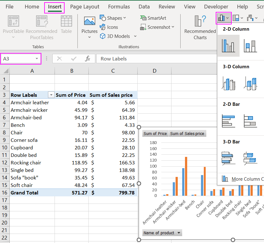
Microsoft Excel will automatically generate a pivot chart and add buttons and other data control elements for dynamic changes in visualization.
Creating the pivot table itself is a bit more involved.
Filter in the Excel Pivot Table
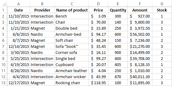
You can convert almost any range of data in the Pivot Table: the results of financial transactions, information about suppliers and buyers, the home library catalog, etc.
For example, take the following table:
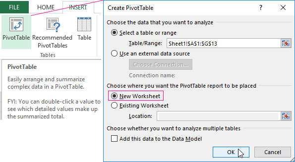
We will create a summary table: "INSERT" - "PivotTable". Put it on a new sheet.
We added information about suppliers including quantity and cost. Now it’s in our consolidated report.
Let's remind how the summary report dialog box looks like:
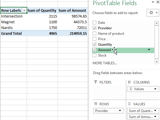
We set the program instructions to generate a summary report while dragging the headers. If you accidentally make an error, you can delete the header from the bottom area or replace it with another one.
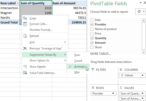
Totals appears according to the data which are placed in the field "Values". In automatic mode it’s the sum. But you can set "average", "maximum", etc. If you need to do this for the values of the entire field, then click on the name of the column and change the way the totals are presented:
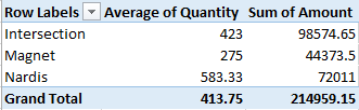
For example, the average number of orders for each supplier:
Results can be changed not in all columns but only in a separate cell. Then we right-click on this cell.
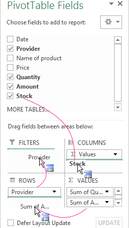
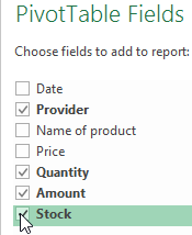
Set the filter in the summary report:
- Put a tick in front of the "Stock" header in the list of fields to add to the table filters we need.
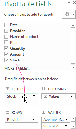
- Drag this field to the "FILTERS" area.
- The table became three-dimensional and the "Stock" tag turn up at the top.
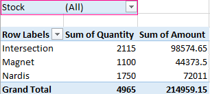
Now we can filter the values in the report by warehouse number. Click on the arrow in the right corner of the cell and select the items we are interested in:
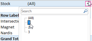
For example, "1":
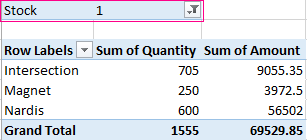
The report displays information only for the first warehouse. We see above the value and the icon of the filter.
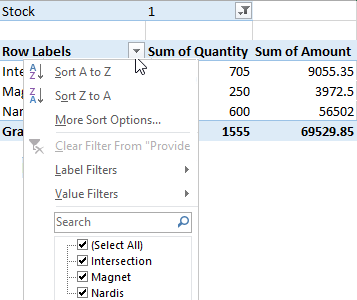
You can also filter the report using the values in the first column.
Sorting in the Excel Pivot Table
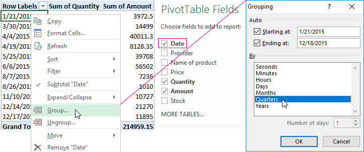
Let's transform our consolidated report: we will remove the value "Suppliers" and add the "Date" tag.
Let's make the table more useful. We will group the dates by quarters. To do this right-click on any cell with a date. In the drop-down menu select "Group". Fill in the grouping parameters:
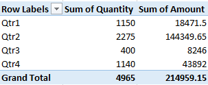
The Pivot Table takes the following form after clicking OK:
Let’s sort the data in the report by the value of the column "Amount". Click the right mouse button on any cell or column name. Select "Sort" and sorting method.
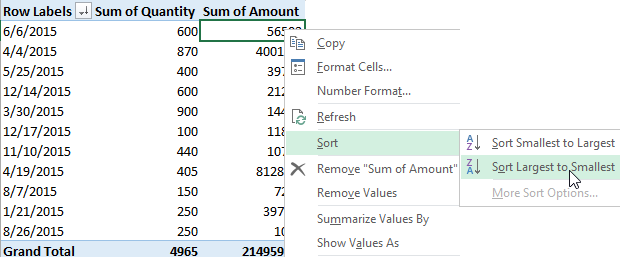
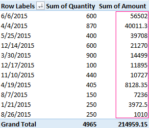
The values in the summary report will be changed according to the sorted data:
Now let's sort the data by date. Click right mouse button and choose "Sort". You can select the sorting method and stop with this step. But we will follow an otherwise pathway. Click "More Sort Options"-"More Options…". A window like this will open:
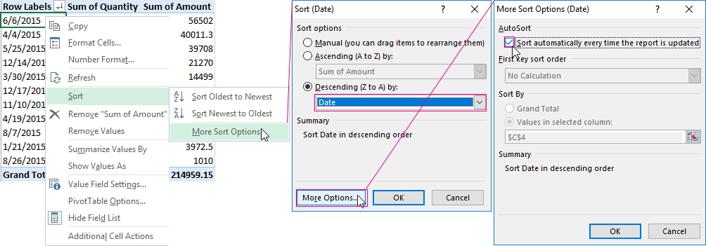
Let's set sorting parameters: "Sort Date in descending order". Click on the "More Options" button. Put a checkmark next to "AutoSort"-"Sort automatically every time the report is updated".
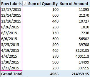
Now Excel will sort dates in descending order (from new to old) when the new dates will appear in the Pivot Table:
Formulas in Excel Pivot Table
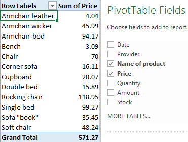
Firstly, we will compile a consolidated report, where the totals will be presented not only by the sum. Let's start from scratch with an empty table. For one we learn how to add a column in the Pivot Table.
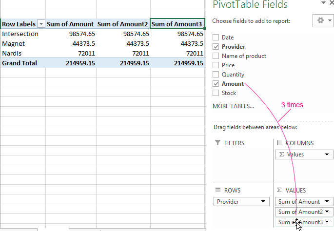
- Add the "Provider" header to the report. We will drag "Amount" header for three times in the "Value" field. Now three identical columns will be added to the Pivot Table.
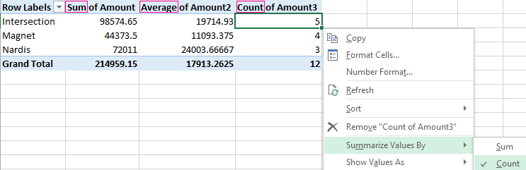
- Leave the value "Sum" for totals in the first column. For the second one choose "Average". For the third one set "Count".
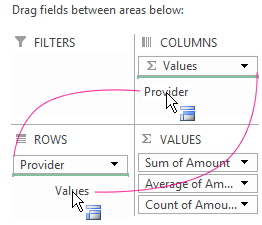
- We swap column values and row values. "Provider" goes to the column names. "Σ values" goes to the lines names.
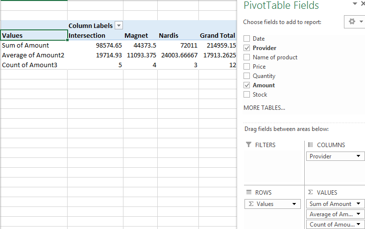
The consolidated report became more convenient for perception:
Let’s study how to prescribe formulas in a summary table. Click on any cell in the report to activate the "PIVOTTABLE TOOLS" tool.
On the "ANALYZE" tab we select "Fields, Items and Sets" - "Calculated Field".
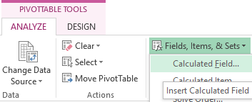
Click and a dialog box opens. Enter the name of the calculated area and the formula to find the values.
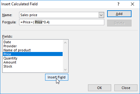
We get the added additional column with the result of calculations using the formula.
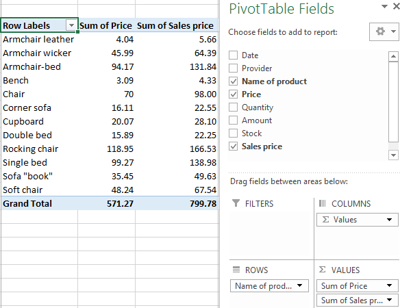
Make an experiments: summary table tools are hothouse. You can always delete the unsuccessful version and redo it If something does not work out.
