Excel Pivot Table training with step-by-step instructions
Pivot Tables in Excel are a powerful tool and one article is not enough to describe all its features and feasibilities. A whole book needed to describe all abilities of summary tables. In this article will be a review of the principled properties of the Pivot Table. In a nutshell, its main feature is a capacity to create all sorts of reports using different summing sets. This definition is difficult to perceive in words, so we immediately turn to examples and practices.
Working with consolidated tables in Excel
Create a table of initial data about the clients of the company as shown in the picture:
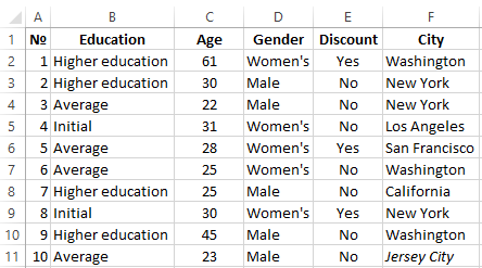
Now we will build a summary table based on the original customer database in which you can easily display the average age of all the clients of the firm who do not have a discount with the separation into:
- age;
- education;
- gender.
Solution for building a consolidated report in Excel:
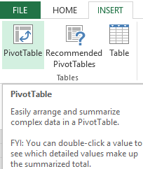
- Go to any cell in the source client database and select the tool: “INSERT” – “Tables” – “PivotTable”.
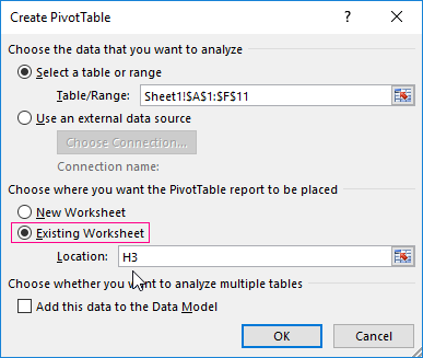
- In the dialog box switch to the "Existing Worksheet" option and specify the value of H3 in the "Location" H3 field:
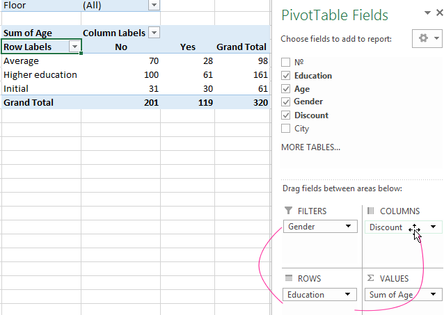
- In the settings window (on the right side) "PivotTable Fields" move the value "Gender" from the "Choose fields to add report:" field into the "FILTRES".
- In the same way distribute the remaining values in the fields as it indicated in the screenshot above.
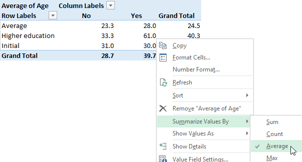
- Right-click on any cell inside the summary table. In the appeared contextual menu select the option: "Summarize Values By" - "Average".
- Round off all values to tenths using the cell format.
Note! In cell I1 we are able to specify the gender (male, female or both) for segmenting the report. It will help make report more descriptive.
Helpful advice! This Pivot Table does not have a dynamic database connection to the clients’ source table. Therefore, any change in the source table is not automatically updated in the summary table. Therefore, after each change of the source data you should right-click on the Pivot Table and select the option "Refresh". Then all the data will be recalculated and updated.
Example with configuring consolidated reports
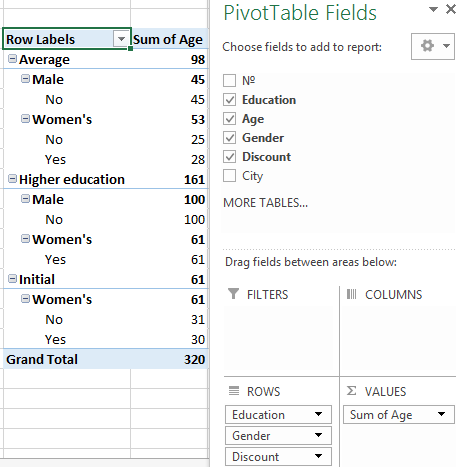
Now we change the structure of the report using the same Pivot Table with the same data.
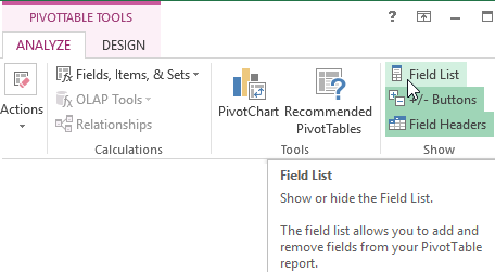
- If you accidentally closed the “PivotTable Fields” window, then left-click on the summary table to make it active. Then enable the option: "PIVOTTABLE TOOLS" - "ANALYZE" - "Show" - "Field List".
- Move the "Gender" value in the "ROWS" field under the "Education" value.
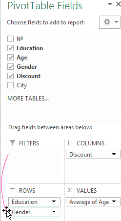
The structure of the report has been radically changed because we add more lines to the fields list:
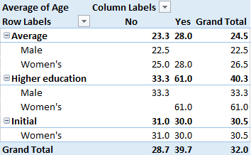
There are groupings that are controlled by buttons (+ and -). These auxiliary buttons and headers can be enabled / disabled through the menu: "PIVOTTABLE TOOLS" - "ANALYZE" -"Show"-"Buttons" or "Field Headers". Also, we no longer have a filter for segmenting the report by gender in cell I1.
