What is Pivot Table in Excel with examples for beginners

Users create PivotTables for analyzing, summarizing and presenting large amounts of data. This Excel tool allows them to filter and group information, as well as display it in different aspects (prepare a report).

PivotTable data source includes a table with several dozens and hundreds of rows, several tables in one workbook, several files. Let's revise the order of PivotTable creation: «INSERT» – «Tables» – «PivotTables».

In this article, we'll learn how to work with PivotTables in Excel.



How to make a pivot table from multiple files

The first step is transferring the information to Excel and transforming it into Excel tables. If our data is in Word, we transfer it to Excel and make a table according to all Excel rules (we give headings to columns, remove empty rows, etc.).

Further work on creating a PivotTable from several files will depend on the type of data. If you work with the same-type data (there are several tables, but the headers are the same), the PivotTable Builder will help you.

We simply create a consolidated report (a PivotTable report) based on data in several ranges of consolidation.

It is much more difficult to make a PivotTable on the basis of source tables that have different structure. For example:

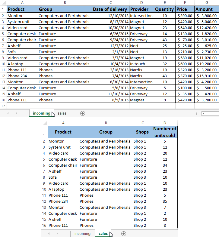
The first table “incoming” represents the receipt of goods. The second “sales” one demonstrates the number of units sold in different stores. We need to combine these two tables in one report to illustrate residues, sales, revenue, etc.

The PivotTable Wizard generates an error with these initial parameters, since one of the main consolidation conditions (the same column names) is violated.

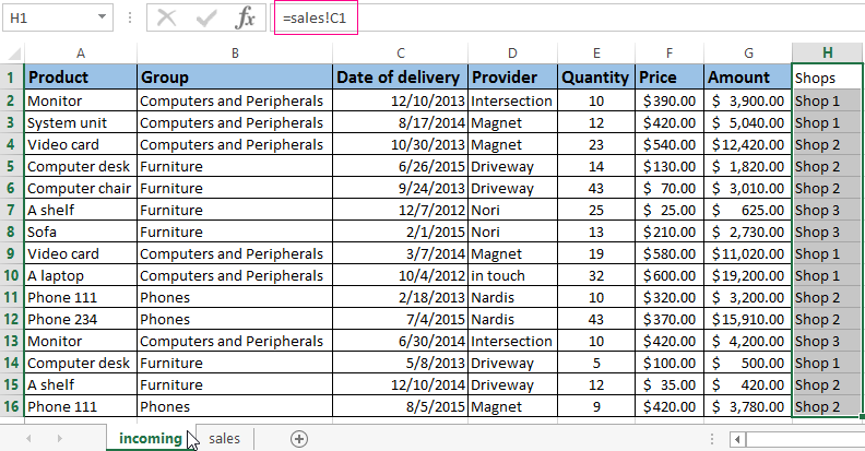
But the two headings in these tables are identical. Therefore, we can combine the data, and then create a summary report.

1. Place the cursor to the target cell (where the table will be moved). Write = - pass to a sheet with the transferred data - select the first cell of a column that is copied. Press Enter. "Multiply" the formula by pulling it down behind the lower right corner of the cell.

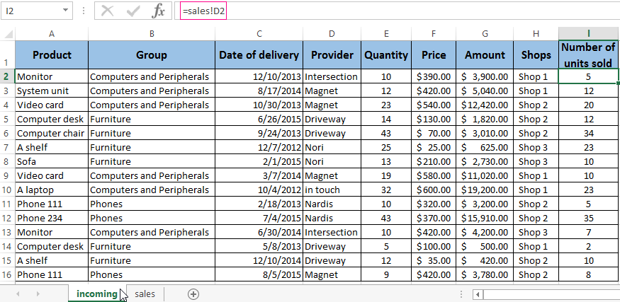
2. We transfer other data by the same principle. As a result, we get one PivotTable from two tables.

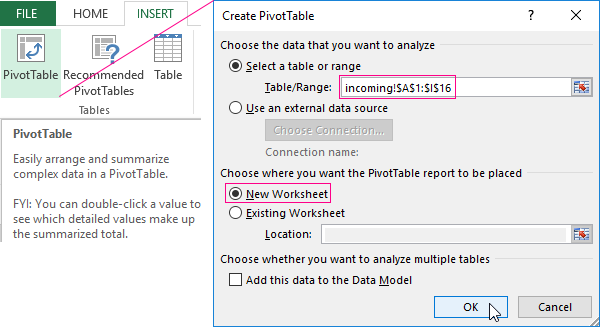
3. Now create a PivotTable report. INSERT – PivotTables - specify the range and location - OK.

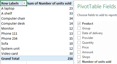
Summary report blank with Fields that can be displayed is opened. Let's show, for example, the quantity of the goods sold.

You can output different parameters for analysis and move fields. But the work with PivotTables in Excel does not end there: capabilities of this tool are wide.



Detailing of information in pivot tables

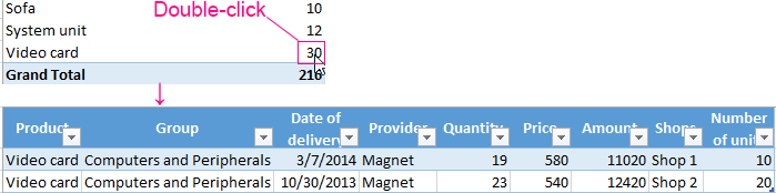
From the report (see above) we can observe that there are 30 video cards sold IN TOTAL. To find out what data was used to get this value, double-click on the number “30”. Get a detailed report:

How to update the data in an Excel PivotTable?

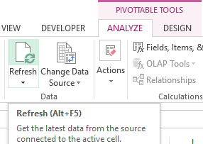
If you change any parameter in the source table or add a new record, this information will not be displayed in the PivotTable report. This situation does not suit us. We choose “PIVOTTABLE TOOL” - “ANALYZE” - “Refresh” (ALT+F5). The cursor must be in any cell in the master report.

Data update:

Or, right-click – refresh.

To configure the automatic update of the PivotTable when changing the data, we do the following:

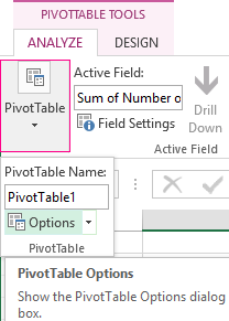
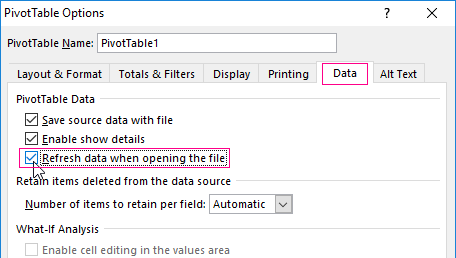
1. The cursor is positioned anywhere in the report. “PIVOTTABLES TOOL” – “ANALYZE” – “PivotTable” – “Options”.

2. In the opened dialog – Data – Refresh data when opening the file – OK.

Change of the structure of the report

Add new fields to the PivotTable:

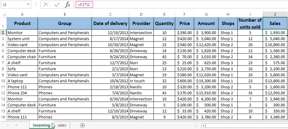
1. Insert the «Sales» column on the sheet with source data. Here we will reflect what revenue the store will receive from the sale of the goods. Let's use the formula - the price (F2) * the number of units sold(I2).

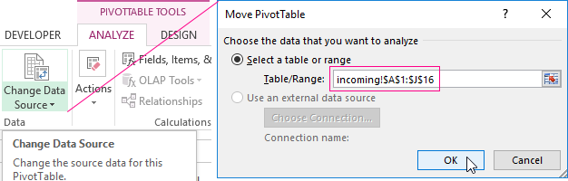
2. Go to the sheet with the report. “PIVOTTABLE TOOL” – “ANALYZE” – “Change Data Source”. Expand the range of information that should enter into the summary table.

If we added columns inside the source table, it was enough to update the PivotTable.

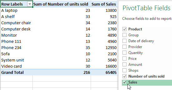
After the range was changed, the «Sales» field appeared in the summary

How to add a calculated field to the PivotTable?

Sometimes, data in the summary table isn’t enough for the user. Changing the initial information does not make sense. In such situations, it is better to add a calculated field.

This is a virtual column created as a result of calculations. It can display average values, percentages, discrepancies, that is the results of different formulas. The data of the calculated field interacts with the data of the PivotTable.

Instructions for adding a calculated field:

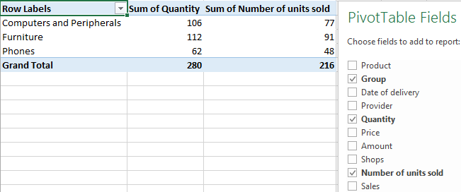
1. Determine what functions the digital column will perform. Define the data in the PivotTable on which the calculated field should refer to. Suppose you need balances for groups of goods.

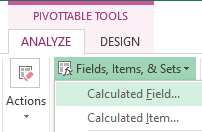
2. “PIVOTTABLE TOOL” – “ANALYZE”–“Fields, Items and Sets”–“Calculated Field”.

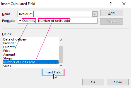
3. Enter the name of the field in the opened menu. Put the cursor in the «Formula» line. The «Calculated Field» tool doesn’t respond to ranges. Therefore, it is pointless to select cells in the PivotTable. Choose the categories that are needed in the calculation from the proposed list. Then click «Insert Field». Complement the formula with the required arithmetic operations.

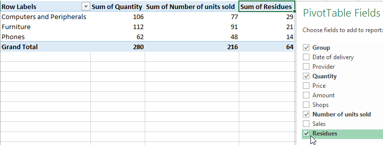
4. Click OK. The Residues appeared.

Grouping data in a consolidated report

For example, we calculate expenses on goods in different years: how much money was spent in 2012, 2013, 2014 and 2015? The grouping by date in the Excel PivotTable is performed as follows. For example, let's make a simple summary by date of delivery and price.

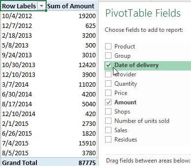
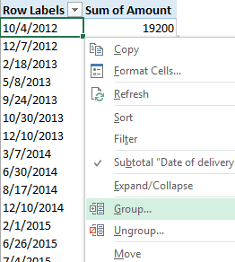
Right-click on any date. Select the «Group» command.

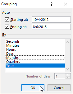
Specify the grouping parameters in the opened dialog. The start and end date of the range are displayed automatically. Choose the «Years» step value.

You’ll receive the amount of orders by years.

Download working example

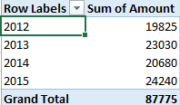
By the same scheme, you can group the data in the PivotTable by other parameters.