Advanced filter in Excel and examples of its features
The information can be displayed in several parameters using the data filtering in Excel. For this purpose, two tools are intended: an auto filter and an advanced filter. They do not delete, but hide data that does not fit the condition. Autofilter performs simple operations. This tool has many more features.
Autofilter and advanced filter in Excel
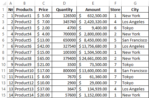
There is a simple table, not formatted and not declared by the list. You can enable the automatic filter through the main menu.
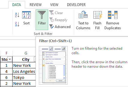
- Select any cell within the range with the mouse. Go to the «DATA» tab and press the «Filter» button.
- Next to the headings of the table, there are arrows that open the lists of the autofilter.
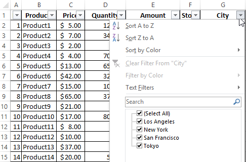
If you format the data range as a table or declare it as a list, the auto filter will be added immediately.
To use the auto-filter is a simple thing: you just need to select an entry with the desired value. For example, display the supplies to the store number. We put the tick in front of the corresponding filtering condition:
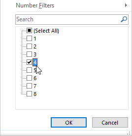
You can see the result immediately:
Peculiarities of the tool:
- AutoFilter works only in an unbroken range. Different tables on one sheet cannot be filtered, even if they have the same type of data.
- The tool treats the top line as column headers and these values are not included in the filter.
- It is acceptable to apply several filtering conditions at once. But each previous result can hide the records necessary for the next filter.
An extended filter has many more features:
- You can set as many conditions for filtering as you want.
- The criteria for selecting the data are visible.
- The user easily finds the unique values in a multi-line array with the help of the advanced filter.
How to make an advanced filter in Excel
A ready-made example is how to use the advanced filter in Excel:
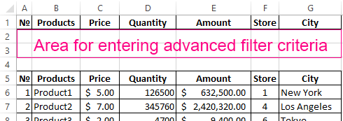
- Create a table with the selected conditions. To do this, copy the headers of the source list and insert it above. In the table with the criteria for filtering, we leave a sufficient number of rows plus an empty string separating from the original table.
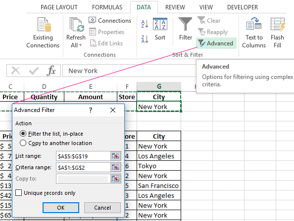
- We will set the filtration parameters for the selection of rows with the value «New York» (in the corresponding column of the table with the terms we enter name city – New York). Activate any cell in the source table. Go to the «DATA» tab - «Advanced».
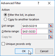
- Fill in the filtering parameters. The initial range is the table with the original data. Links appear automatically, because one of the cells was active. A range of conditions is a condition label. Exit the Advanced menu by clicking OK.
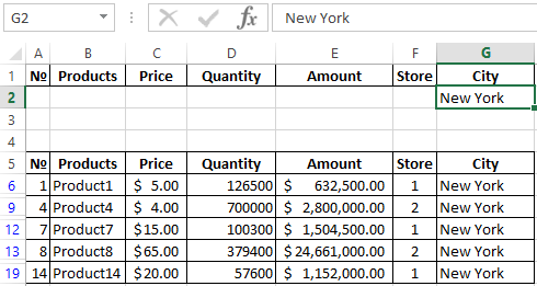
Only the lines containing the value «New York» remained in the source table. To cancel the filter, we should click the «Clear» button in the «Sort» section.
How to use the advanced filter in Excel
Consider using the advanced filter in Excel to select the lines containing the words «New York» or «Los Angeles». The conditions for filtering must be in the same column. It is each under another in our example.
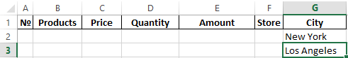
Fill in the advanced filter menu:
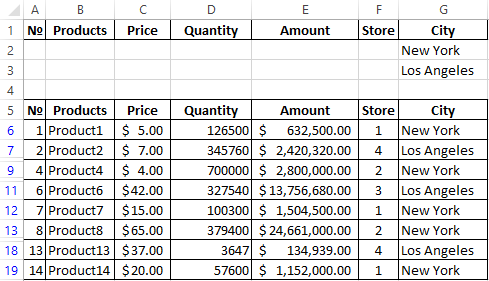
We get the table with the rows selected according to the specified criteria:
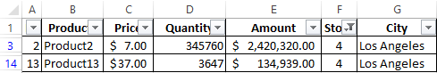
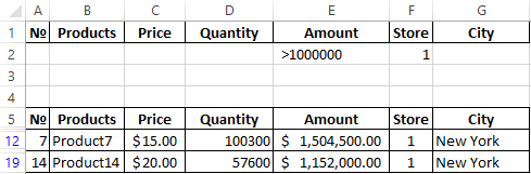
We will select the rows that contain the value «1» in the «Store» column, and the column value "> 1 000 000$". The criteria for filtering must be in the appropriate columns of the condition label in one line. Fill in the filtering parameters. Click OK.
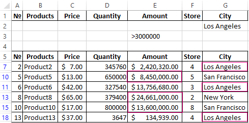
Leave in the table only those lines that contain the word «Los Angeles» in the column «City» or in the column «Amount» - the value ">3 000 000$". Since the selection criteria apply to different columns, we place them on different lines under the appropriate headings. Apply tool:
This tool can work with formulas, which allows the user to solve almost any task when selecting values from arrays.
Fundamental rules:
- The result of the formula is a selection criterion.
- The recorded formula returns the result TRUE or FALSE.
- The initial range is indicated by absolute references, and the selection criterion (in the form of a formula) is using the relative references.
- If TRUE is returned, the string will be displayed after applying the filter. FALSE is not.
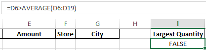
We display rows containing an amount above the average. For this purpose, aside from the table with the criteria (in cell I1), we will enter the name «Largest Quantity». Below is the formula. We use the AVERAGE function.
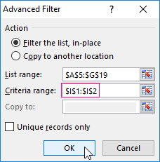
Select any cell in the original range and call the tool. As a criterion for the selection we indicate I1: I2.
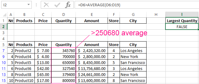
Only those rows are left in the table, where the values in the «Quantity» column are above the average.
To leave only non-repeating lines in the table, in the «Advanced Filter» window put the birdie in front of «Unique records only».
Download advanced filter example
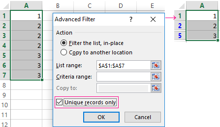
Click OK. Duplicate rows will be hidden. Only unique records remain on the sheet.
