Advanced filter in Excel using filtration of data

Advanced filter in Excel provides more opportunities for managing on data management spreadsheets. It is more complex in settings, but much more effective in action.

Using a standard filter, a Microsoft Excel user can solve not all of the tasks that are set. There is no visual display of the applied filtering conditions. It is not possible to apply more than two selection criteria. You can not filter the duplicate values to leave only unique records. And the criteria themselves are schematic and simple. The functionality of the extended filter is much richer. Let's take a closer look at its possibilities.



How to make the advanced filter in Excel?

The advanced filter allows you to analysis data on an unlimited set of conditions. With this tool, the user can:

• to specify more than two selection criteria;
• to copy the result of filtering to another sheet;
• to set the condition of any complexity with the helping of formulas;
• to extract the unique values.

The algorithm for applying the extended filter is simple.

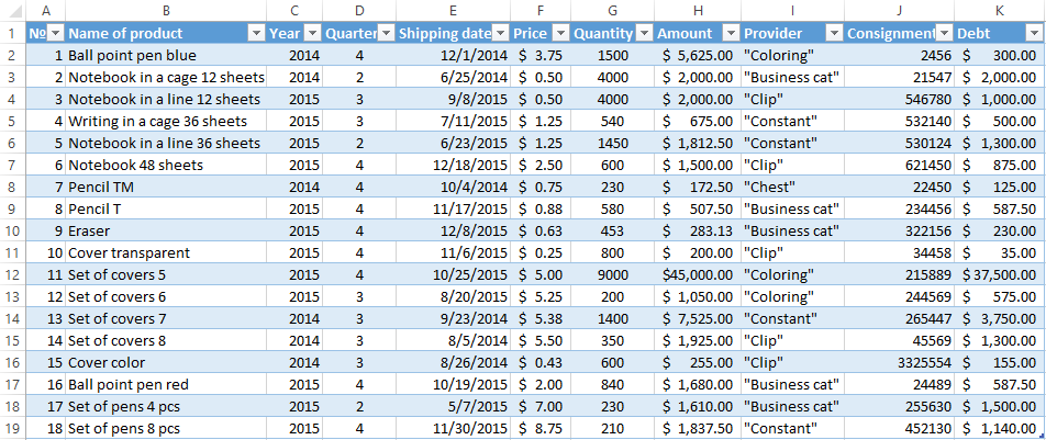
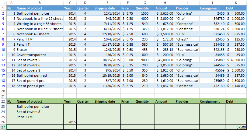
1. To make the table with the original data or to open an existing one. Like so:

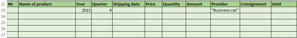
2. To create the condition table. The features: the header line is the same with the «cap» of the filtered table. To avoid errors, need to copy the header line in the source table and paste it on the same sheet (side, top, underarm) or on another sheet. We enter the selection criteria into the condition table.

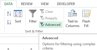
3. Go to the «DATA» tab - «Sort and filter» - «Advanced». If the filtered information should be displayed on another sheet (NOT where the source table is), then you need to run the extended filter from another sheet.

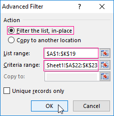
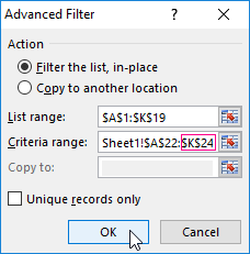
4. In the «Advanced Filter» window that opens, to select the method of processing information (on the same sheet or on the other one), set the initial range (the table 1, example) and the range of conditions (the table 2, conditions). The header lines must be included in the ranges.

5. To close the «Advanced Filter» window, click OK. We see the result.

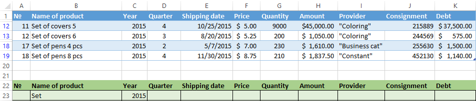
The top table is the result of the filtering. The lower nameplate with the conditions is given for clarity near.



How to use the advanced filter in Excel?

To cancel the action of the advanced filter, we place the cursor anywhere in the table and press Ctrl + Shift + L or «DATA» - «Sort and Filter» - «Clear».

We will find using the «Advanced Filter» tool information on the values that contain the word «Set».

In the table of conditions we bring in the criteria. For example, these are:

The program in this case will search for all information on the goods, in the title of which there is the word «Set».

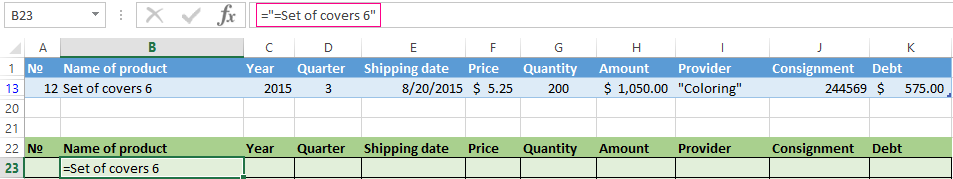
To search for the exact value, you can use the «=» sign. We enter the following criteria in the condition table:

Excel sees the «=» as a signal: the user will set the formula now. In order for the program to work correctly, the following should be written in the formula line: ="=Set of covers 6".

After using the «Advanced Filter»:

We filter the source table by the condition «OR» for different columns now. The operator «OR» is also in the tool «AutoFilter». But there it can be used within the single column.

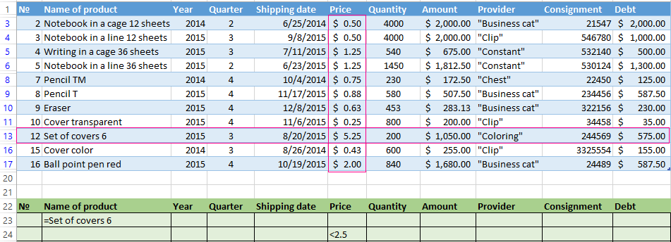
In the condition label we introduce the selection criteria: ="=Set of covers 6". (In the column «Name of product») and = «<2.5$» (in the column «Price»). That is, the program must select those values that contain the EXACTLY information about the good «Set of covers 6 ». OR to the information about the goods, which price is <2.5.

Please note: the criteria must be written under the corresponding headings in the DIFFERENT lines.

The result of selection:

The advanced filter allows you to use as a criterion of a formula. Let's consider the example.

Selection of the line with the maximum indebtedness: =MAX(Table1[Debt]).

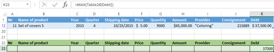
So we get the results as after running several filters on the one Excel sheet.

How to make few filters in Excel?

Let's create the filter by several values. To do this, we enter in the table of conditions several criteria for selecting data:

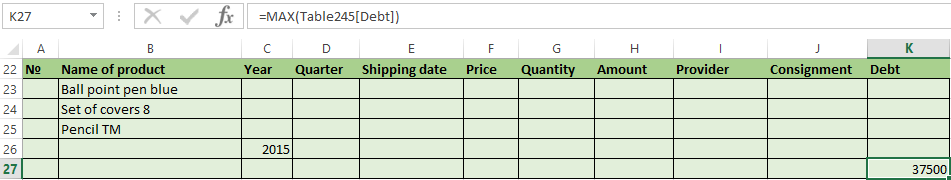
Apply the tool «Advanced Filter»:

Now from the table with the selected data we will extract new information, which was selected according to other criteria. There are only shipping date for autumn 2015 (from September to November). Example:

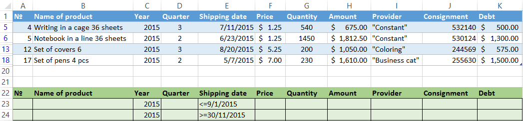
We introduce a new criterion in the condition table and apply the filtering tool. The initial range - is the table with data selected according to the previous criterion. This is how the filter is performed across on several columns.

To use few filters, you can create several condition tables on the new sheets. The method of implementation depends from the task which was set by user.

How to make the filter in Excel by lines?

By standard methods - you may not do it by any ways. Microsoft Excel selects data only in columns. Therefore, we need to look for other solutions.

Here are some examples of string criteria for the extended filter in Excel:

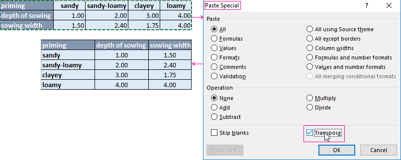
1. Convert to the table. For example, from three rows make a list of three columns and apply the filtering to the transformed version.

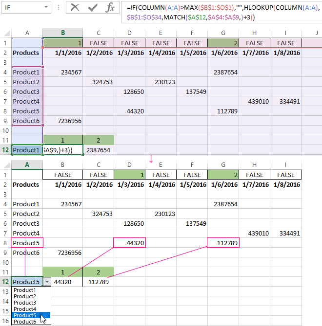
2. Use formulas to display exactly the data in the string that are needed. For example, make some indicator drop-down list. And in the next cell, enter the formula using the IF function. When a certain value is selected from the drop-down list, its parameter appears next to it.

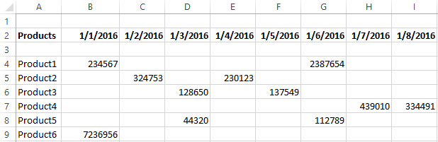
To give an example of how the filter works by rows in Excel, we are creating the label:

For the list of products, we create the drop-down list:

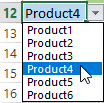
If necessary, learn how to create a drop-down list in Excel.

Above the table with the original data, we insert an empty line. In the cells, we introduce the formula that will show which columns the information is taken from.

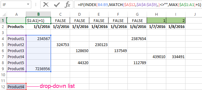
Next to the drop-down list box, we enter the following formula:

Its task is select from the table those values, that correspond to a certain good.

Download examples of advanced filtering

Thus, using the tool "Drop-down list" and built-in functions Excel selects data in rows according to a certain criterion.