Sorting the data in Excel in rows and columns using formulas
Sorting the data in Excel is a tool for presenting information in a user-friendly form. Numerical values can be sorted in ascending and descending order, text values can be sorted alphabetically and in reverse order. Available options are the sorting by color and font, in random order, according to several conditions. Columns and rows are sorted.
Sorting order in Excel
There are two ways to open the sort menu:
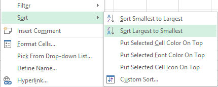
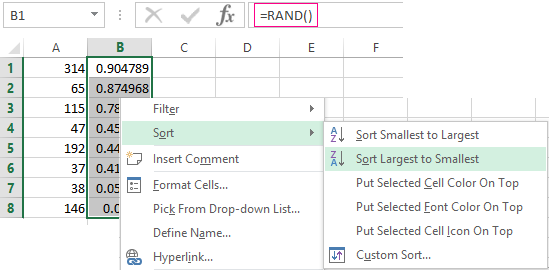
- Right-click on the table. Select «Sort» and method «Largest to Smallest».
- Open the «DATA» tab - «Sort» dialog box.
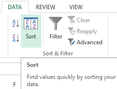
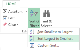
Frequently used sorting methods are represented by a single button on the «HOME» tab «Editing» section.
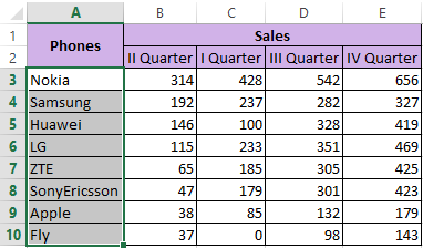
Sorting the table by a separate column:
- For the program to perform the task correctly, select the required column in the data range.
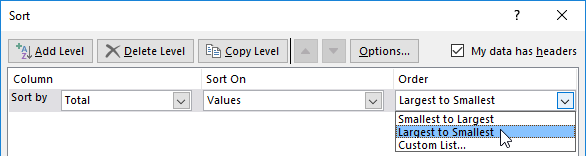
- Then we act in accordance with the task. If you want to perform simple sorting in ascending / descending order (alphabet or vice versa), just click the corresponding button on the taskbar. When the range contains more than one column, Excel opens a dialog box like:
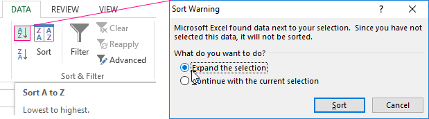 To maintain the correspondence of the values in the lines, we select the action "Expand the selection". Otherwise, only the selected column is sorted - the structure of the table is broken.
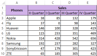
If you select the entire table and sort it, the first column is sorted. Data in the rows will be in accordance with the position of the values in the first column.
Sorting by the cell color and font
Excel provides rich formatting capabilities to the user. Therefore, it is possible to operate in different formats.
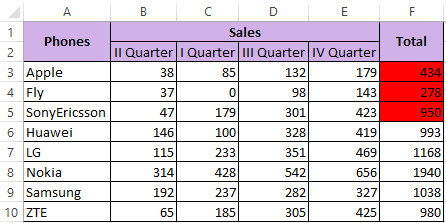
We will make the column «Total» and "fill" the cells with values in different shades in the training table. Perform the color sorting:
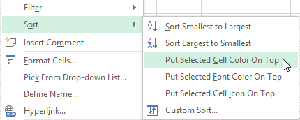
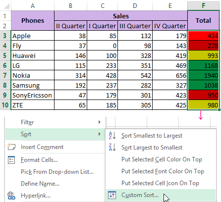
- Select the column - the right mouse button - «Sort».
- From the proposed list, select «Put Selected Cell Color On Top».
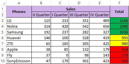
- We agree to "Expand the selection". Result:
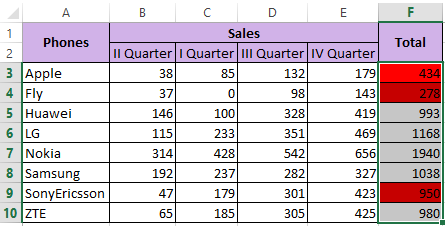
The program sorted cells by accents. The user can choose the order of the color sorting. For this purpose, in the list of tool options, select «Custom Sort».
In the window that opens, enter the required parameters:
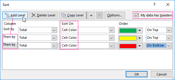
Here you can choose the order of the representation the cells of different colors.
By the same principle, the font data is sorted.
Sorting by multiple columns in Excel
How to set the order of secondary sorting in Excel? To solve this problem, you need to set several sorting conditions.
- Open the menu «Custom Sort». Assign the first criterion.
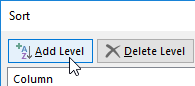
- Click the button «Add Level».
- There are windows for entering data for the next sorting condition. We fill them.
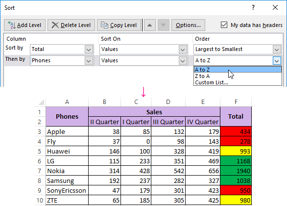
The program allows you to add several criteria at once to perform the sorting in a special order.
Sorting the rows in Excel
By default, the data is sorted by columns. How to sort by rows in Excel:
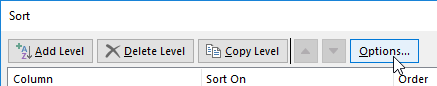
- In the «Custom Sort» dialog box, click the «Options» button.
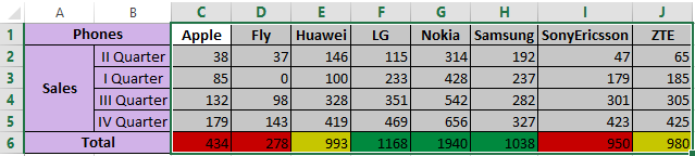
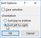
- In the menu that opens, select «Range Columns».
- Click OK. In the «Sort» window, fields for filling in the conditions for the rows appear.
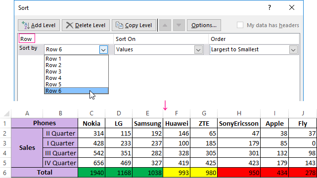
Thus, the table is sorted into Excel by several parameters.
Random sorting in Excel
The built-in sorting options do not allow you to arrange data in a column randomly. This task will be handled by the function =RAND().
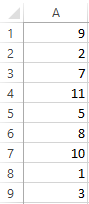
For example, you need to arrange a set of certain numbers in a random order.
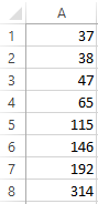
We put the cursor in the next cell (left-right, not important). In the formula row, enter =RAND(). Press Enter. We copy the formula to the whole column - we get a set of random numbers.
Now sort the resulting column in ascending / descending order - the values in the original range will automatically be placed in random order.
Dynamic table sorting in Excel
If you apply standard sorting to the table, then when you change the data, it will not be relevant. You need to make sure that the values are sorted automatically. We use formulas.
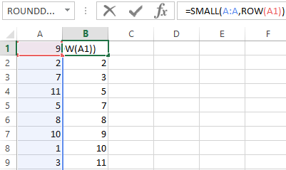
- There is a set of primes that need to be sorted in ascending order.
- Put the cursor in the next cell and enter the formula: =SMALL(A:A,ROW(A1)). Exactly, as a range we specify the whole column. And as a coefficient there is the function of SMALL() ROW() with reference to the first cell.
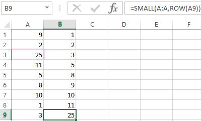
- Lets change the number in the initial range to 7 to 25 - "sorting" ascending will also change.
If it is necessary to make the dynamic sorting in descending order, use the =LARGE() function.
To sort the text values dynamically, you need the array formulas.
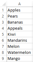
- Initial data is a list of some names in any order. In our example it is a list of fruits.
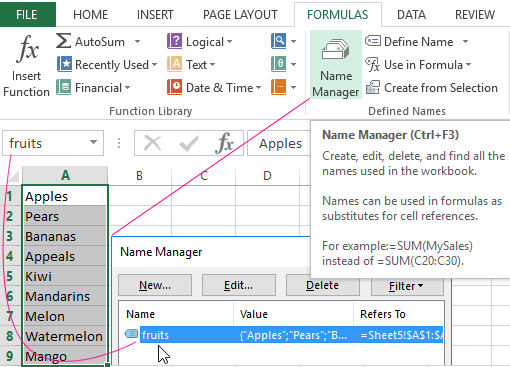
- Select the column and give it the name «fruits». To do this, in the field of names that is near the formula line, enter the name we need to assign it to the selected range of cells.
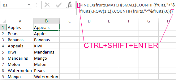
- In the next cell (in the example - in B1), we write the formula: Since we have an array formula before us, press Ctrl + Shift + Enter. We multiply the formula by the whole column.
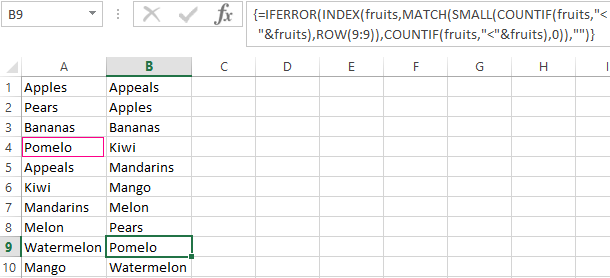
- If lines are added to the original column, then we introduce a slightly modified formula:
Add the "pomelo" value to the "fruit" name range and check:
Download sorting data in excel using formulas
Subsequently, when you add data to the table, the sorting process will be performed automatically.
