Chart of funnel sales in Excel download for free

The sales funnel – is the tool for analyzing and optimizing the business process. The concept describes and demonstrates the psychology of the consumer. Not all people who see the advertising of the product will become real customers. Some of the potential buyers are not interested in the goods. Part - will go to competitors. The rest part can not be arranged by the price.

How to calculate the number of consumers of a product to make a business profitable? How to collect statistics on sales? The funnel allows you to control all these processes.



The functional capabilities of the instrument

1. The meaningful control over the transition process of a potential buyer to a transaction.
2. The visualize of conversion for each stage. You can see how the sales funnel fills in - you can analyze the effectiveness of the promotion channel.
3. You can predict how to fill out the stages in a month, two, three... On the basis of forecasts, a sales volume plan is drawn up for each manager, for the enterprise as a whole.
4. The sales funnel allows you to analyze the performance of each manager, sales department.

Stages of the funnel

Number and content depend on the type of business. In diagram form the sales funnel looks like an inverted pyramid. The symbolic demonstration of the «entrance-exit» of customers: not all people interested in the product will reach the purchase. A part of potential buyers will refuse from the transaction at this or that stage.

At each stage work their own laws, that determine to the behavior of a manager in relation to the potential consumer of the goods. The task of any stage is to bring the client to the next step.

In general, the funnel includes the following sections:

1. The widest part –there is potential customers (everyone who saw the advertisement, learned about the product, went to the site, etc.).
2. All those customers, with whom the first contact happened (call, meeting, presentation, registration on the site, etc.).
3. Customers who are interested in the product (there is feedback from them).
4. Clients who have concluded the contract.
5. Customers who paid for the product (payment confirms that the transaction is completed).

Data is taken from the results of statistical studies, sales department reports, managers, databases.



How to make the sales funnel in Excel

There are no ready-made tools for creating the funnel in Excel. Nevertheless, it can be done.

First, we'll make the nameplate with statistical data:

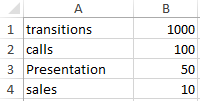
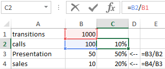
The next step – we calculate the conversion at each stage. To do this, we divide the value of the current section by the value of the previous one and in the cell with the result we set the percentage format:

Next, you need to go to the «Insert» tab - SmartArt drawings. Of the proposed options, the most obvious is the «Pyramid».

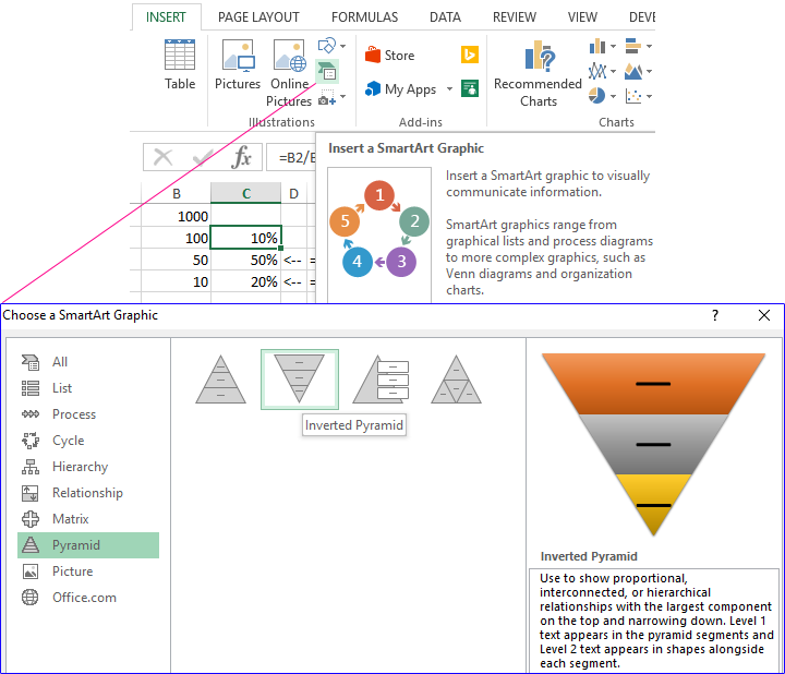
The standard pyramid with three elements is appeared.

There are 4 sections in our example – so let's add one more element. Put the cursor in the text area and press Enter.

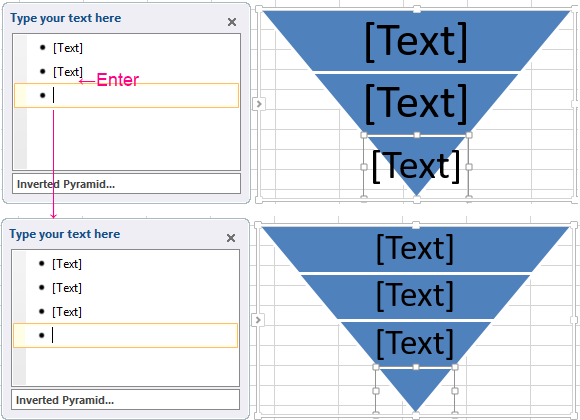
You can enter any text - at this stage it does not matter. Automatically, another element appears in the pyramid.

Change Colors, select: «SMARTART»-«DESIGN»-«Change Colors»-«Colorful – Accent Colors».

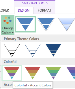
The preliminary layout is ready. You can play with colors, styles. For example, to make the pyramid three-dimensional.

In the next step, we combine the cell values in the A column (names of sections) with the cell values in the B column (the quantitative expression of the sections). We do this with the ampersand symbol.

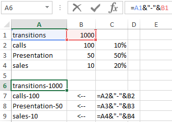
To substitute this data in the layout, you need to convert the object in the SmartArt format to a regular shape. Without this step, we will not be able to automatically update the shape when making changes to the table.

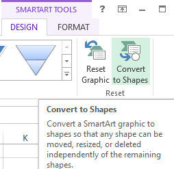
To do this, click the «Convert to Shapes» button on the «SMARTART»-«DESIGN» tab.

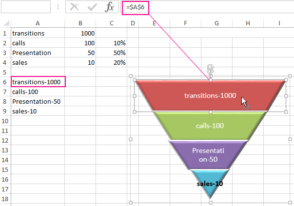
Now take turns clicking on each cell – we click on the line of formulas – we make the link to the merged cell. We get such the simple funnel:

Consider how to calculate the sales funnel in Excel in another way.

For example, let's take another table of values:

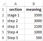
Using the REPEAT function, we create the following figure:

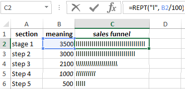
All values are 100%. The function has put as many predefined elements as the proportion of each value in the total value.

Let's give to the diagram a familiar look of the funnel:

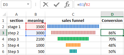
This effect can be achieved with font formatting and alignment.

The diagram «Funnel sales» in Excel

We use the same table with data. We select the range A2:B6. Go to the «Insert» tab. In the «Charts» group we select «3-D 100% Stacked Column».

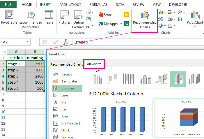
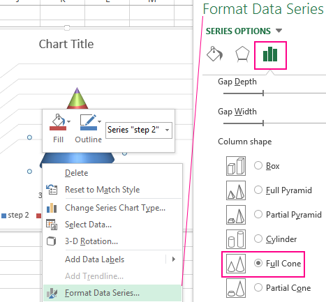
Right-click on the diagram. Choose the «Format Data Series» and check the box opposite the «Full Cone».

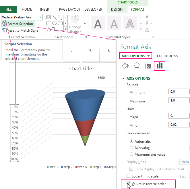
Next, we go to the «CHART TOOLS»-«Format» tab. We find the «Current Selection» menu, open the list and select the «Vertical (Value) Axis». The next step is to open the «Format Selection»-«Format Axis»-«AXIS OPTIONS». We select to the vertical axis of values and to tick the «Values in reverse order».

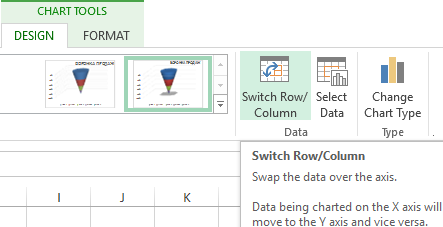
If necessary, to merge all the cones into one with the accumulation of indicators, go to the «Working with diagrams» menu, then to the «CHART TOOLS»-«DESIGN» tab and click on the «Switch Row/Column» tool to swap the values of the axes.

We add the data captions. We remove the grid, the legend, the axes and format it at our discretion.

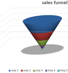
We get the funnel of sales. When you make changes to the table, the height of the funnel elements will change automatically.

Funnel sales in Excel free download

The notation. If you need to make a flat diagram, then on the «Rotate the 3D shape» tab we set the X and Y axes to zero values.