Solving equations in Excel using the Cramer and Gauss iterations method
There is an extensive toolkit in Excel for solving different types of equations by different methods. Let's look at some solutions using examples.
Solving equations by trial and error method in Excel
The tool "Goal Seek" is used in a situation when the result is known but arguments are unknown. Excel picks up the values until the computation yields the desired total.
The path to the command: «DATA» - «Data Tools» - «What-if-Analysis» - «Goal Seek».
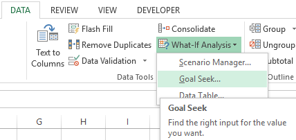
Let’s consider, for example, the solution of the quadratic equation x2 + 3x + 2 = 0. The order of finding the root with Excel:
- We enter into the cell B2 a formula for finding the value of the function. We apply a reference to cell B1 as an argument.
- Open the menu of the "Goal Seek" tool. In the box "Set cell" is a reference to cell B2 where the formula is located. Enter 0 in the "To value" field. This is the value that you want to get. In the column "By changing cell" is B1. The selected parameter should be displayed here.
- After clicking OK, the result of the selection is displayed. If you want to save it click OK again. Otherwise, click "Cancel".


The program uses a cyclic process to find a parameter. You need to enter the Excel parameters to change the number of iterations and the error.
Set the maximum number of iterations and the relative error on the "Formulas" tab. Set a checkmark in the box to enable iterative calculations.
How to solve the system of equations by using the matrix method in Excel?
A system of equations is given:
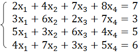
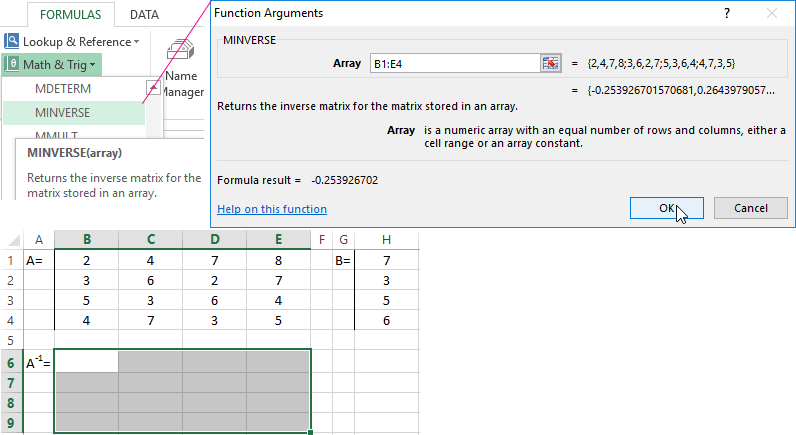
- We enter the values of the elements in Excel cells in the form of a table.
- Let us find the inverse matrix. Select the range B6:E9 where the matrix elements will later be placed (we are guided by the number of rows and columns in the original matrix). Open the list of functions (fx). In the category "Math and Trig" we find the MINVERS function. The argument is an array of cells with elements of the original matrix.
- Click OK and a value appears in the upper left corner of the range. Consecutively press the F2 button and Ctrl + Shift + Enter.
- We multiply the inverse matrix Ax-1x by the matrix B (only in this order of multiplication!). We select the range H1:H4 where the elements of the resulting matrix will subsequently appear (we are guided by the number of rows and columns of the matrix B). Open the dialog box of the MMULT mathematical function. The first range is the inverse matrix. The second one is the matrix B.
- Close the window with the arguments of the function by clicking OK. Consistently press the F2 button and the combination Ctrl + Shift + Enter.

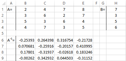
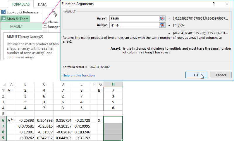
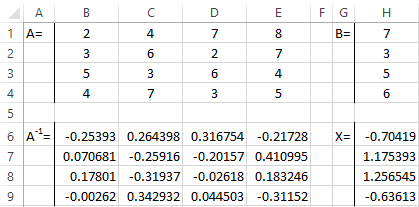
The roots of the equations are obtained.
Solving the system of equations by the Cramer method in Excel
We take the system of equations from the previous example:

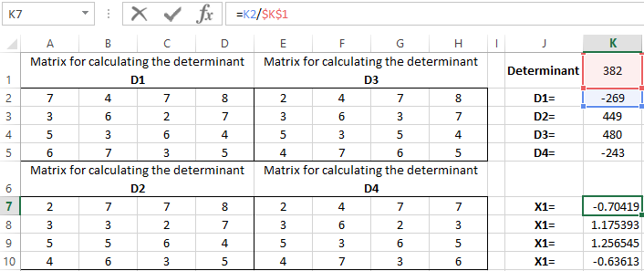
We calculate the determinants of the matrices obtained by replacing one column in the matrix A by the column matrix B. And it will be solved by using the Cramer method.
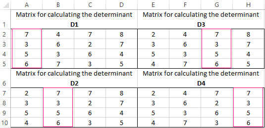
Use the MDETERM function to calculate the determinants. The argument is a range with the corresponding matrix.
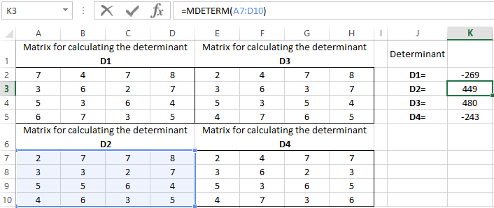
We also calculate the determinant of the matrix A (the array is the range of the matrix A).
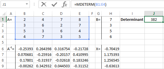
The determinant of the system is greater than 0 and the solution can be found by the Cramer formula (Dx / |A|).
For the calculation of Х1: =K2/$K$1, where K2 is D1. For the calculation of Х2: =K3/$K$1, and etc. We get the roots of the equations:
Solving the systems of equations by using the method of Gauss in Excel
For example, let's take the simplest system of equations:
3а + 2в – 5с = -1
2а – в – 3с = 13
а + 2в – с = 9
We write the coefficients in the matrix A. And write the constant term in the matrix B.

For clarity, the free terms will be selected by flood filling. You need to swap the lines if in the first cell of the matrix A was 0 so that there will be a value which differs from 0.
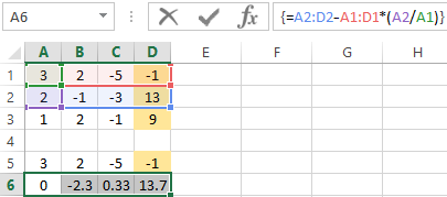
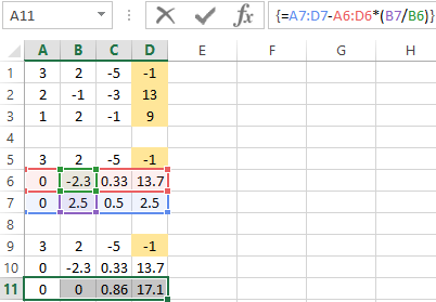
- We give the 0 to all the coefficients of the matrix A except the first equation. We copy the values in the first row of two matrices to cells B6:E6. In cell B7 we enter the formula: Then select the range B7:E7. Press F2 and press Ctrl + Shift + Enter. We subtracted from the second line the first one which is multiplied by the ratio of the first elements of the second and first equation.
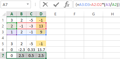
- Copy the entered formula on row 7. So we got rid of the coefficients before A. Only the first equation was retained.
- We reduce to 0 all the coefficients of B in the third and fourth equations. We copy lines 5 and 6 (only values). Then we transfer them below in lines 9 and 10. These data should remain unchanged. Then we enter the formula of the array in cell A11
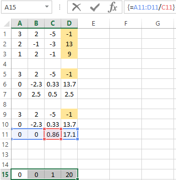
- A direct run was done by Gauss's method. In the reverse order, we start running from the last row of the resulting matrix. All the elements of this line must be divided by a factor of C. Enter the array formula in the line:
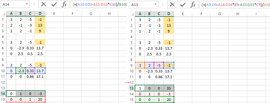
- In line 15: we subtract the third line from the second one, multiplied by the coefficient C from the second line In line 14: from the first line we subtract the second and third one, multiplied by the corresponding coefficients In the last column of the new matrix, we get the roots of the equation.
Examples of solving equations by using the iteration method in Excel
The calculations in the workbook should be configured as follows:

This can be done on the "Formulas" tab in the "Excel Options". Let’s find the root of the equation х – х3 + 1 = 0 (а = 1, b = 2) by iteration using cyclic references. Formula:
Хn+1 = Xn– F (Xn) / M, n = 0, 1, 2, … .
M is the maximum value of the derivative modulo. We perform the calculations to find M:
f’ (1) = -2 * f’ (2) = -11.
The resulting value is less than 0. Therefore, the function will have the opposite sign: f (х) = -х + х3 – 1. М = 11.
We enter the value in cell A1: a=1. Accuracy is three decimal places. Then we enter the formula to calculate the current value of x in an adjacent cell (B1):

We control the value of f(x) in cell C1 using the formula:

Download solving equations in Excel
The root of the equation is 1. We enter the value 2 into cell A1. We obtain the same result. There is only a single root in the given interval.
