Subtotals in Excel with examples of functions
You can sum up the subtotals in the Excel table using the built-in formulas and the corresponding command in the «Structure» group on the «Data» tab.
The important condition of using tools – the values are organized in the form of a list or a database, the same records are in the same group. When you create the summary report, the subtotals are generated automatically.
Calculation of subtotals in Excel
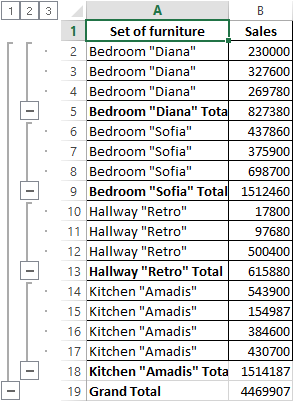
To demonstrate the calculation of subtotals in Excel, let's take the small example. We suppose that a user has a list with the sales of certain goods:
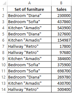
It is necessary to calculate the revenue from the sale of certain groups of goods. If you use a filter, you can get the same type of records according to the specified selection criteria. But the values will have to be calculated manually. Therefore, we will use another Microsoft Excel tool – the «Interim Results» command.
In order for the function to produce the correct result, check the range for the following conditions:
- The table is organized in the form of the simple list or database.
- The first line - shows the column names.
- The columns contain the same values.
- There are no empty rows or columns in the table.
Let's start ...
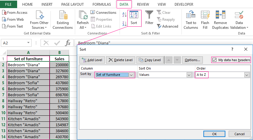
- We sort the range by the value of the first column - the same type of data should be near.
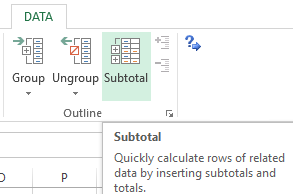
- Select any cell in the table. Select the «DATA» tab on the line. The group «Outline» – is the team «Subtotal».
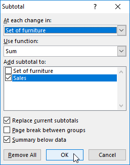
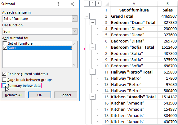
- We fill the dialog box in the «Subtotal». In the field «At each change in» we select the condition for data selection (in this example, «Value»). In the field «Use function:» we assign the function «Sum». In the «Add subtotal to» field, you should mark the columns to which the function will apply (Sales).
- Close the dialog box by clicking OK. The initial table acquires the following form:
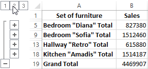
If you collapse the rows in the subgroups (click on the «minus» to the left of the line numbers), then we get the table only from the subtotals:
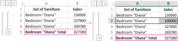
Each time the column «Set of furniture» is changed, the subtotal is recalculated in the «Sales» column.
In order for each intermediate result to be followed by a page break, in the dialog box you need to tick the «Page break between groups».
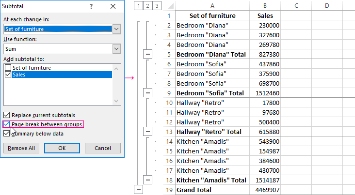
In order for intermediate data to be displayed OVER the group, remove the «Summary below data» condition.
The team subtotals allows you to use several statistical functions simultaneously. We have already designated the operation «Sum». Add the average sales for each group of products.
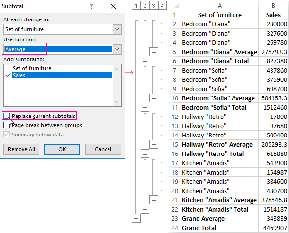
We call the menu «Subtotals» again. We remove the tick «Replace current subtotals», and in the «Use function:» field, select «Average».
Formula «Subtotals» in Excel: the examples
The «INTERMEDIATE» function returns the subtotal in the list or in the database. Syntax: the number of function, the reference 1; the reference 2;...
The number of function - is a number from 1 to 11, which shows the statistical function for calculating subtotals:
- AVERAGE (the average arithmetic)
- ACCOUNT (the number of cells)
- COUNTAIN (the number of non-empty cells)
- MAX (maximum value in the range)
- MIN (the minimum value)
- COMPOS (product of numbers)
- STDEV (standard deviation from the sample)
- STDEVP (standard deviation of the population)
- SUM
- DISP (variance in production)
- DISPP (population variance)
The reference 1 – is the mandatory argument indicating the named range for finding the subtotals.
The features of the «work» function:
- outputs the result by explicit and hidden lines;
- excludes lines not included in the filter;
- counts only in columns, for rows not suitable.
Consider using the function as an example:
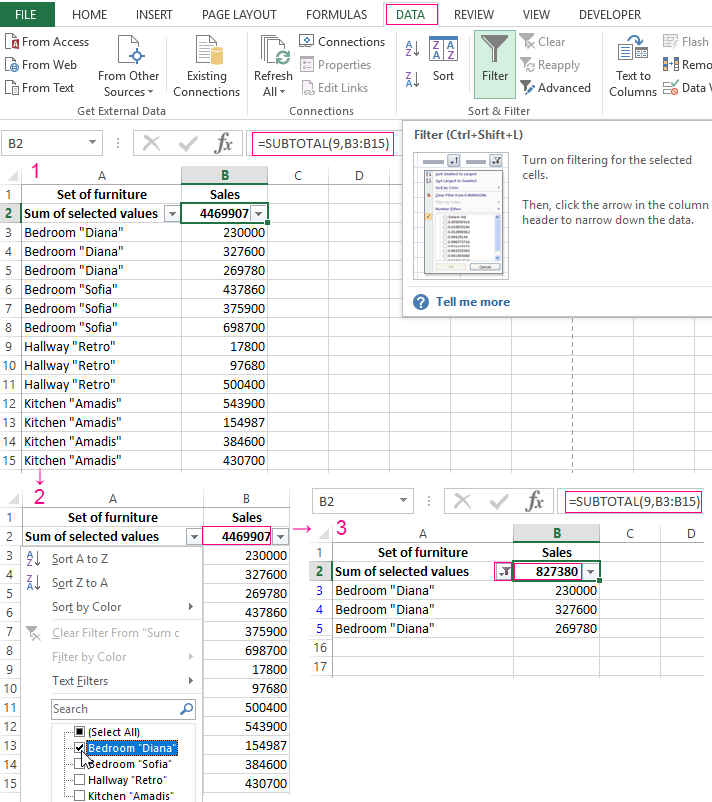
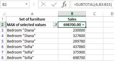
- Create the additional line for displaying subtotals. For example, there is «Sum of selected values».
- Turn on the filter. Let's leave in the table only the data on the value of the Kitchen «Amaids».
- In the cell B2 we introduce the formula =SUBTOTAL():
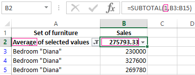
The formula for the average value of the intermediate total of the range:
The formula for the maximum value (for bedrooms):
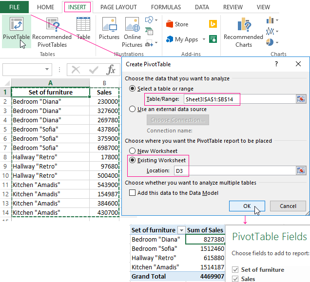
Subtotals in the Excel Pivot Table
In the summary table, you can show or hide subtotals for rows and columns.
- The automatic summation function for calculation of totals is already included the formation of the consolidated report.
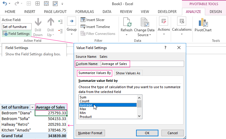
- To apply another function, in the «PIVOTTABLE TOOL» section on the «ANALYZE» tab, we find the «Active Field» group. The cursor must be in the cell of the column whose values the function will be applied to. Press the button «Field Setting». In the menu that opens, select «Average». Assign the desired function to the subtotals.
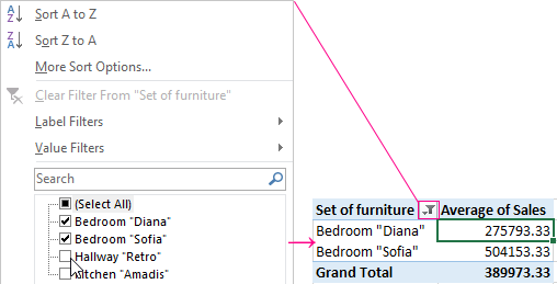
- To display totals for individual values, use the filter button in the right corner of the name of column.
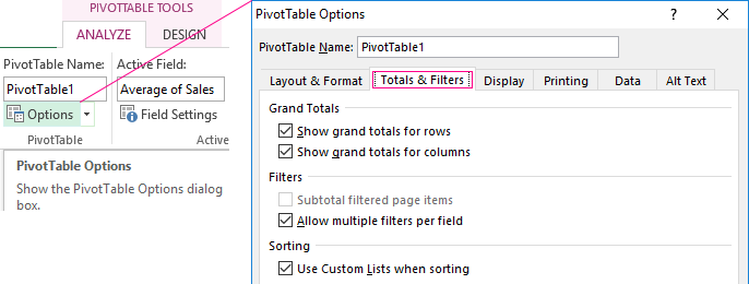
In the «PIVOTTABLE TOOL» menu «ANALYZE»-«PivotTable»-«Options», the «Totals and Filters» tab is available.
Download examples of subtotals
Thus, to display subtotals in Excel lists, three methods are used: the command of the «DATA»-«Outline» group, the built-in function and the summary table.

Data Visualization Charts for Interactive Report Creation in Excel.
Dashboard Templates