How to build a chart on a table in Excel: step by step instruction
Any information is easier to perceive when it's represented in a visual form. It's particularly relevant for numeric data that needs to be compared. In this case, charts are the optimal variant of representation. We will work in Excel.
Moreover, we will learn to create dynamic charts and graphs, which are updated automatically when you change the data. The link at the end of the article will allow you to download a sample template.
How to build a chart off a table in Excel?
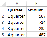
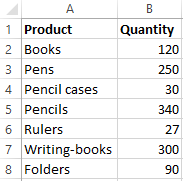
- Create a table with the data.
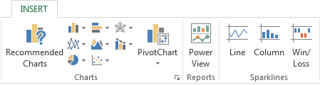
- Select the range of values A1:B5 that need to be presented as a chart. Go to the «INSERT» tab and choose the type.
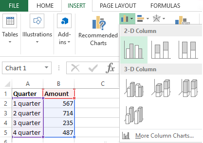
- Click «Insert Column Chart» (as an example; you may choose a different type). Select one of the suggested bar charts.
- After you choose your bar chart type, it will be generated automatically.
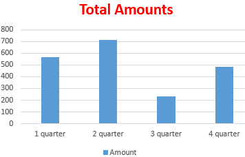
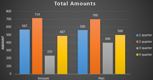
- Such a variant isn't exactly what we need, so let's modify it. Double-click on the bar chart's title and enter «Total Amounts».
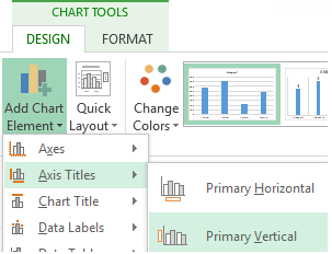
- Add the vertical axis title. Go to «CHART TOOLS» - «DESIGN» - «Add Element» - «Axis Titles» - «Primary Vertical». Select the vertical axis and its title type.
- Enter «AMOUNT».
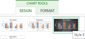
- Change the color and style. Choose a different style number 9.
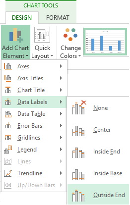
- Specify the sums by giving titles to the bars. Go to the «DESIGN» tab, select «Data Labels» and the desired position.
Done!
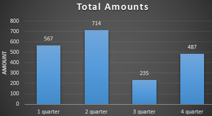
As a result, we have a stylish presentation of the data in Excel.
How to add data in an Excel chart?
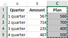
- Add new values to the table – the «Plan» column.
- Select the new range of values, including the heading. Copy it to the clipboard (by pressing Ctrl+C). Select the existing chart and paste the fragment (by pressing Ctrl+V).
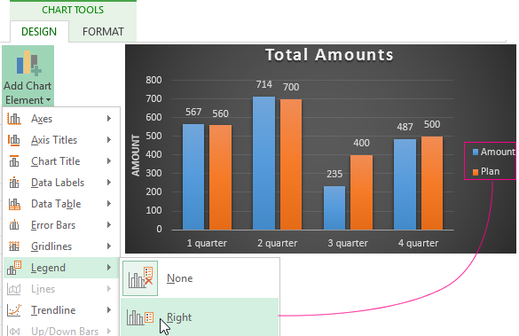
- As it's not entirely clear where the figures in our bar chart come from, let's create the legend. Go to «DESIGN» - «Legend» - «Right». This is the result:
There is a more complicated way of adding new data into the existing graph through the «DESIGN» «Select Data» menu (open it by right-clicking and selecting «Select Data»).
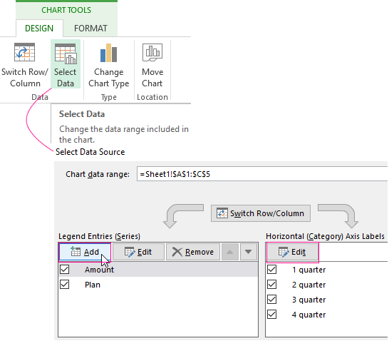
After you click «Add» (legend elements), there will open the row for selecting the range of values.
How to reverse axes in an Excel chart?
In the menu you've opened, click the «DESIGN»-«Switch/Column» button.
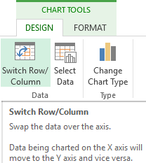
The values for rows and categories will swap around automatically.
How to lock controls in an Excel chart?
If you need to add new data in the bar chart very often, it's not convenient to change the range every time. The optimal variant is to create a dynamic chart that will update automatically. To lock the controls, let's transform the data range into a «Smart Table».
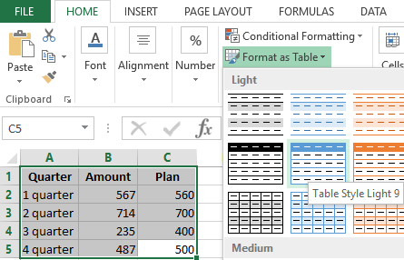
- Select the range of values A1:C5 and click «Format as Table» on «HOME» tab.
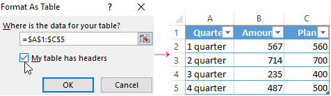
- Select any style in the drop-down menu. The program suggests you select the range for the table – agree with the suggested variant. The values for the graph will appear as follows:
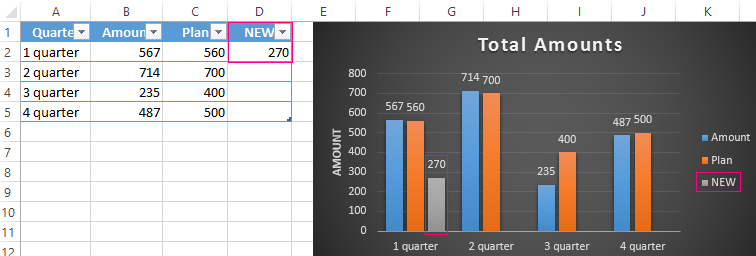
- As soon as you begin to enter new information in the table, the chart will also change. It has become dynamic:
We have learned how to create a «Smart Table» off the existing data. If the spreadsheet is blank, start off with entering the values in the table: «INSERT» - «Table».
How to build a percentage chart in Excel?
Pie charts are the best option for representing percentage information.
The input data for our sample chart:
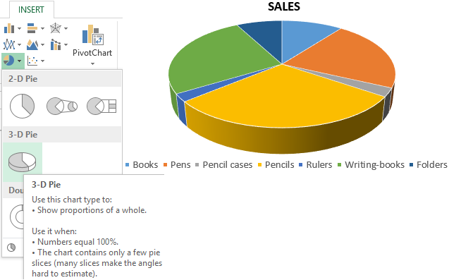
- Select the range A1:B8. «INSERT» - «Insert Pie or Doughnut Chart» - «3D-Pie».
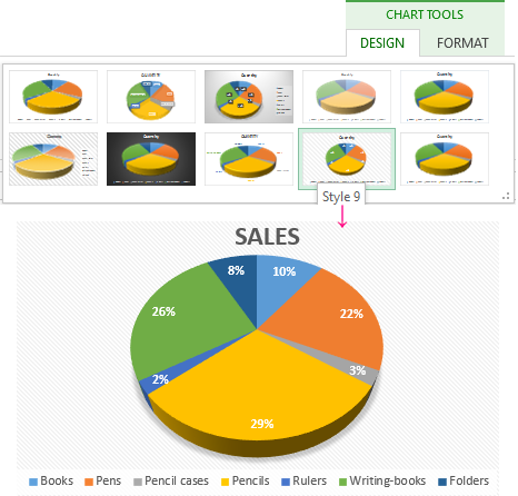
- Go to the tab «DESIGN» - «Styles». Among the suggested options, there are styles that include percentages. Choose the suitable 9.
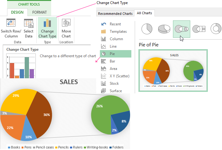
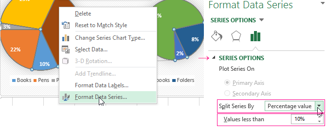
- The small percentage sectors are visible poorly. To highlight them, let's create a secondary chart. Select the pie. Go to the tab «DESIGN» - «Change Chart Type». Select a pie with a secondary graph.
- The automatically generated option does not fulfill the task. Right-click on any sector. The dots designating the boundaries will become visible. Click «Format Data Series». Enter the following row parameters:
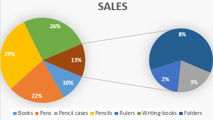
- We have obtained the desired variant:
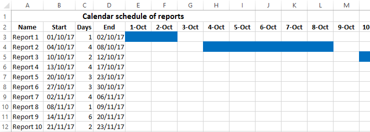
Gantt chart in Excel
The Gantt chart is way of representing information in the form of bars to illustrate a multi-stage event. It's a simple yet impressive trick.
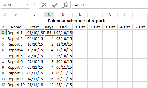
- We have a (dummy) table containing the deadlines for different reports.
- To create a chart, insert a column containing the number of days (column C). Fill it in with the help of Excel formulas.
- Select the range to contain the Gantt chart (E3:BF12). That is, the cells to be filled with a color between the beginning and end dates.
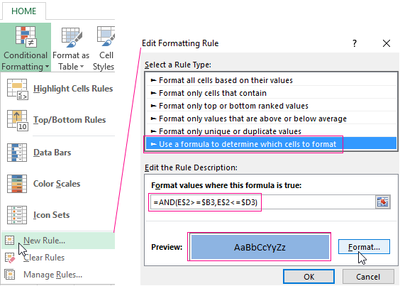
- Open the «Conditional Formatting» menu (on the «HOME» tab). Select «New Rule» - «Use a formula to determine which cells to format».
- Enter the formula of the following type: =AND(E$2>=$B3,E$2<=$D3). Excel uses the operator «И» to compare the date in the current cell with the beginning and end dates. Then, click «Format» and select the fill color.
When you need to build a presentable financial report, it's better to use the graphical data representation tools.
A simple Gantt graph is ready. You can also download the template with a sample:
If the information is represented in a graphical way, it's perceived visually much quicker and more efficiently than texts and numbers. It makes it easier to conduct an analytic analysis. It makes the situation clearer – both the whole picture and particular details.
Charts and graphs were specifically developed in Excel for fulfilling such tasks.

Data Visualization Charts for Interactive Report Creation in Excel.
Dashboard Templates