How to Create 3D Graphics for Game in Excel Using Formulas

In this article, I will explain how I managed to port a 3D scene rendering algorithm into Excel formulas (without macros). For those unfamiliar with computer graphics, I have tried to describe all the steps as simply and in as much detail as possible. Basically, understanding the formulas should be achievable with high school math knowledge (+ the ability to multiply a 3D matrix by a vector).

Examples of Creating 3D Graphics for a Game in Excel

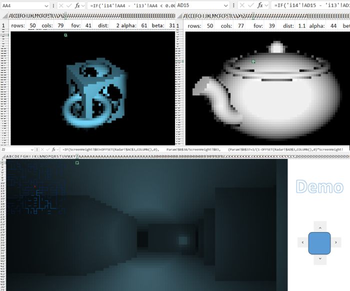
By mastering the information in this article, you will learn to create arbitrary 3D models and even simple 3D games using only Excel formulas, without macros or programming skills. All you need is the ability to work with formulas and functions in Excel. Examples of a 3D game and a model generator for 3D graphics can be downloaded at the end of the article via links to Excel files.

Caution! The article contains a lot of useful material with examples – a total of 20 images and 3 animations below.

In the Excel files available for download at the end of the article, you can modify the following cells:

• alpha: horizontal camera rotation in degrees;
• beta: vertical camera rotation in degrees;
• dist: distance from the camera to the origin;
• fov: camera "zoom".

To rotate the camera, you need to grant Excel permission to edit the file.

If you download your Excel file from ObservableHQ, you must color the cells manually. Highlight all small square cells and select "Conditional Formatting" > "Color Scales."

3D Ray Marching Algorithm in Excel Formulas

The Ray Marching algorithm was popularized by Inigo Quilez in 2008 after his presentation: "Rendering Worlds with Two Triangles" about a compact 3D engine for the demoscene.

Afterward, Inigo Quilez created the Shadertoy website, and most of the works submitted there use the described technique. It turns out that you can create photorealistic scenes with it; take a look, for example, at this: gallery.

Ray Marching is a very simple and efficient algorithm that allows rendering fairly complex scenes. Why, then, is it not used on graphics cards? The thing is, graphics cards are optimized for working with 3D figures composed of triangles, for which Ray Marching is less effective.

Principle of Operation of a 3D Engine for a Game Using Excel Formulas

1. The object is described as a function.
2. Assign a ray emerging from the camera to each pixel of the result.
3. For each ray, find the intersection coordinates with the object.
4. Determine the pixel color based on the intersection point.

I think that, in one form or another, all these subtasks are solved in any 3D engine for creating 3D games.

Object Description

There are three ways to describe a 3D object:

1. An explicit formula that, given a ray emerging from the camera, returns the intersection point with the object (or, for example, the direction of the tangent at it).
2. Membership function. It indicates whether a point in space belongs to the object or not.
3. Real-valued function. For points inside the object, it is negative; outside, it is positive.

In this article, we will use a specific case of the third option, called the signed distance function (SDF).

An SDF takes a point in space as input and returns the distance to the nearest point on the object. For points inside, it equals the distance to the object's boundary with a "minus" sign.

Finding the Intersection of a Ray and a 3D Object

Let's assume we have a ray originating from the camera, and we want to find its intersection point with the object.

Several methods come to mind for finding this point:

1. Iterate over points on the ray with a certain step.
2. Having points inside and outside the object, perform a binary search to refine the intersection location.
3. Or use any root-finding method for the SDF (which is negative inside the object and positive outside), limited to the ray.

But here, we will use another method: Ray Marching.

This is a simple algorithm that only works with SDFs.

Let's parameterize the ray by the distance from its origin with the function: ray(t) = (x,y,z).

Then ray(0) is the camera itself. Here's the algorithm:

• t = 0;
• repeat N times: t = t + SDF(ray(t));
• if t < TMax, return ray(t) as the intersection point, otherwise report that the ray does not intersect the object.

Here N is the number of iterations we can afford.

The larger N, the more accurate the algorithm.

The number TMax is the distance from the camera within which we expect to find the object.

Principle of the 3D Graphics Generation Algorithm in Excel

Will the algorithm always reach the intersection point with the object (or, more precisely, converge towards it)? An object may have a complex shape, and other parts of it may closely approach the ray, preventing the algorithm from converging to the intersection point. In reality, this cannot happen: other parts of the object will inevitably be at some nonzero distance from the ray (otherwise, the ray would intersect them), which we denote as δ<0. Thus, the SDF function will be greater than δ for any point on the ray (except for points very close to the intersection point). Therefore, sooner or later, it will approach the intersection point.

On the other hand, if the algorithm converges to a point, the distance between successive iterations approaches zero ⇒ SDF (the distance to the nearest point of the object) also approaches zero ⇒ in the limit SDF = 0 ⇒ the algorithm converges to the ray-object intersection point.

Obtaining the Pixel Color from the Intersection Point

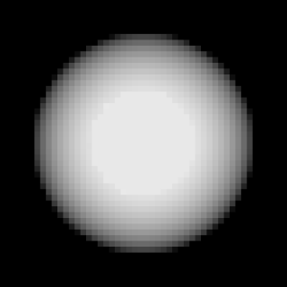
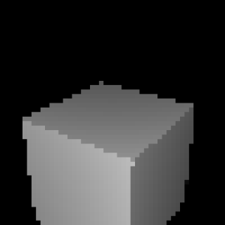
Let's assume that for each pixel, we have found the intersection point with the object. We can render these values (i.e., the distance from the camera to the intersection point) directly and obtain images like these:

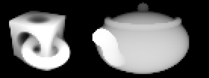
Considering that this was achieved using Excel, it's not bad. But we want to know if we can make the colors more like how we see objects in real life.

In computer graphics, the basic method for calculating color is Phong shading. According to Phong, the final color consists of three components: ambient, specular, and diffuse. Since we are not aiming for photorealistic renders, using just the diffuse component will suffice. The formula for this component follows Lambert's law and states that the pixel color is proportional to the cosine of the angle between the surface normal and the direction to the light source.

Next, to simplify calculations, let's assume the light source and the camera coincide. Then, in essence, we need to find the sine of the angle between the ray from the camera and the object's surface:

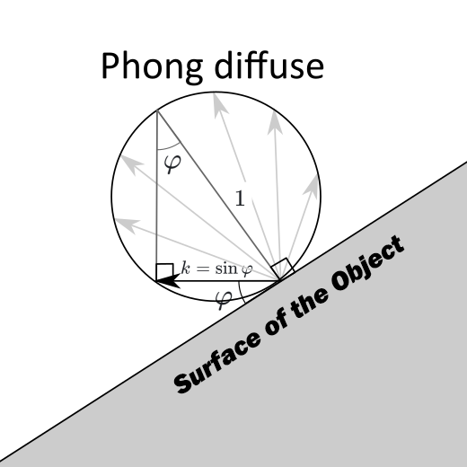
The desired angle Φ is marked with a single arc in the diagram. Its sine value is denoted as k.

Typically, when using the Ray Marching method, to find the surface normal of an object, the SDF value is calculated at six points (it can be reduced to four points) near the intersection point, and the gradient of this function is found, which should match the normal. I found this to be too many calculations for Excel and wanted to find the desired angle more simply.

If you look at the convergence rate of the algorithm, you can notice that if the angle between the ray and the object is perpendicular, only one iteration is needed. If the angle is small, the algorithm will converge very slowly.

Could it be possible to obtain information about the angle to the surface based on the algorithm's convergence rate? If so, no additional calculations would be required: it would be enough to analyze the values of the previous iterations.

Let's draw a diagram. Let I_n and I_n+1 be points obtained in successive iterations of the algorithm. Let's assume the points are close enough to the object that it can be approximated by a plane, whose angle we want to find. Let R = SDF(I_n), r = SDF(I_n+1) be the distances from points I_n and I_n+1 to the plane. According to the algorithm, the distance between I_n and I_n+1 is equal to R.

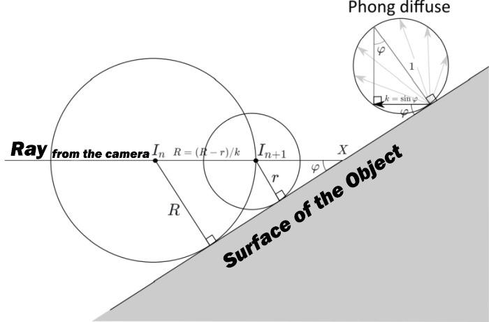
On the other hand, if X is the intersection point of the ray and the figure, then: _InX = R / k, and I_{n + 1}X = r / k. Consequently:

$R=I_n{I}_{n+1}=I_{n}X-I_{n+1}X=\frac{R-r}{k}$

$k=\frac{R-r}{R}=1-\frac{r}{R}=1-\frac{\mathrm{SDF}\left(I_{n+1}\right)}{\mathrm{SDF}\left(I_n\right)}$

That is, the pixel intensity equals one minus the ratio of the SDF values from successive iterations!

Describing Simple Shapes with Formulas

Examples of SDF for a sphere, cube, and torus:

Table of Formulas for Generating 3D Models in Excel
$\sqrt{x^2+y^2+z^2}-r$
$\max \left(\right|x|,|y|,|z\left|\right)-\frac{\mathrm{side}}{2}$
$\sqrt{{\sqrt{x^2+z^2}-R}^2+y^2}-r$

Shapes can be moved and compressed along the axes:

Examples of formulas for modifying 3D models created in Excel
$\mathrm{cube}(x,y+0.3,z)$
$\mathrm{cube}(x,2\cdot y,z)$

Shapes can also be combined, intersected, and subtracted. That is, SDF supports basic constructive solid geometry operations:

Formulas for merging and subtracting 3D models in Excel
min(sphere(x, y, z), cube(x, y, z))
max(sphere(x, y, z), cube(x, y, z))
max(-sphere(x, y, z), cube(x, y, z))

An attentive reader may notice that some shapes (e.g., cubes), as well as some operations (e.g., compression), the given formulas do not always return the distance to the nearest point of the object, meaning they are not formally SDF. Nevertheless, it turns out they can still be input into a 3D SDF engine and it will render them correctly.

This is just a small part of what can be done using SDF.

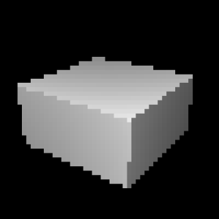
Combining all the given formulas, we get the first shape:

Example of a formula for creating a complex 3D model in Excel

$$\min \left( \max \left(\right|x|-0.3,|y|-0.3,|z|-0.3,-\sqrt{x^2+y^2+z^2}+0.375), \sqrt{{\sqrt{{(x-0.25)}^2+{(z-0.25)}^2}-0.25}^2+y^2}-0.05\right)$$

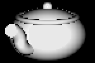
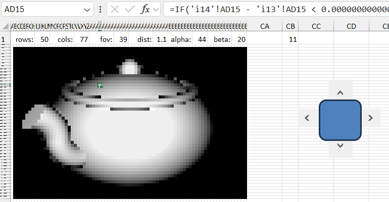
Formula for creating a 3D teapot model

The teapot is a bit more complicated - first, we need a plan:

$$\min ( \sqrt{x^2+{(y-0.27)}^2+z^2}-0.05, \sqrt{x^2+{2.5\cdot y^2}^{}+z^2}-0.4, \sqrt{{\sqrt{x^2+z^2}-0.3}^2+{(y-0.18)}^2}-0.02, \max \left( x+y-0.7, -y+0.09, \sqrt{{\sqrt{{(x-0.55)}^2+{(y-0.09)}^2}-0.1}^2+{(z-0.1)}^2}-0.04\right), \max \left( -(-y+0.09), \sqrt{{\sqrt{{(x-0.35)}^2+{(y-0.09)}^2}-0.1}^2+{(z-0.1)}^2}-0.04\right))$$

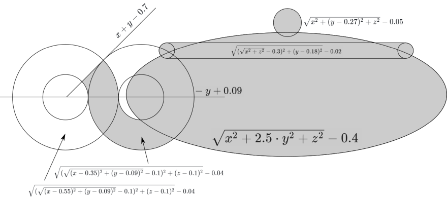
And adjust the angle. Done:

Camera Setup Formulas

All we need to do is find the corresponding ray in space for a given pixel on the screen, emanating from the camera. More precisely, we need to be able to find a point on this ray based on the distance to the camera. This means we need a function ray(s, t, d), where s, t are the pixel coordinates, and d is the distance from the start of the ray (camera).

For calculation convenience, pixel coordinates will be set relative to the center of the screen. Given that the screen consists of $rows$ rows and cols columns, we expect coordinates within the range:

$$s\in [-\frac{\mathrm{cols}}{2},\frac{\mathrm{cols}}{2}],t\in [-\frac{\mathrm{rows}}{2},\frac{\mathrm{rows}}{2}]$$

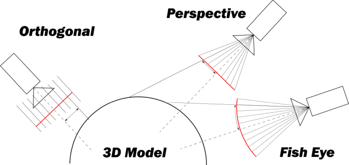
Next, we need to determine the type of camera projection: orthogonal, perspective, or "fish-eye". They are all roughly the same in terms of implementation complexity, but perspective is most commonly used in practice, so we will use it.

Most of the calculations in this chapter could be avoided, for example, by placing the camera at point (1, 0, 0) and directing it along the $X$ axis. But since the shapes are also aligned along the axes, the result would not be a very interesting view. In the case of a cube, we would see it as a square.

To allow the camera to rotate, a careful number of calculations with Euler angles need to be performed. Thus, we get three variables as input: angle alpha, angle beta, and distance dist. They determine both the position and the direction of the camera (the camera always looks at the origin).

Using WolframAlpha, we find the rotation matrix:

$$\left(\begin{array}{c}x\\ y\\ z\end{array}\right)=\underset{\underset{x}{-\left(M\right(\alpha ,\beta \left)\right)}}{\begin{array}{c}\left(\pi ʠ\right)\\ \backslash cos\left(\alpha \right)ʠ\backslash cos\left(\beta \right)-\backslash cos\left(\alpha \right)ʠ\backslash sin\left(\beta \right)& \backslash sin\left(a\right)\\ \backslash sin\left(\beta \right)& \backslash cos\left(\beta \right)& 0\\ -\backslash cos\left(\beta \right)ʠ\backslash sin\left(\alpha \right)& \backslash sin\left(\alpha \right)ʠ\backslash sin\left(\beta \right)& \backslash cos\left(\alpha \right)\end{array}}\angle \begin{array}{c}\mathrm{x\text{'}}\\ \mathrm{y\text{'}}\\ \mathrm{z\text{'}}\end{array}$$

If applied to the vector (dist, 0, 0), we get the camera coordinates (don't ask me where the minus went):

$$\left(\begin{array}{c}\mathrm{camX}\\ \mathrm{camY}\\ \mathrm{camZ}\end{array}\right)=\begin{array}{c}M\\ (\alpha ,\beta )\end{array}\cdot \begin{array}{c}\mathrm{dist}\\ 0\\ 0\end{array}=\mathrm{dist}\cdot \begin{array}{c}\backslash cos\left(\alpha \right)\cdot \backslash cos\left(\beta \right)\\ \backslash sin\left(\beta \right)\\ \backslash sin\left(\alpha \right)\cdot \backslash cos\left(\beta \right)\end{array}$$

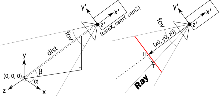
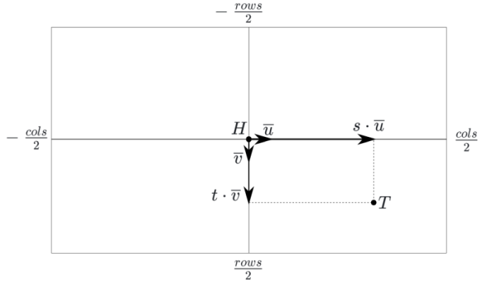
The subsequent calculations will be specific to the perspective projection. The main object is the screen (in the image, it's in red, and in the text, it is italicized). This is an imaginary rectangle at some distance in front of the camera, which, as you might guess, corresponds directly to the pixels on a regular screen. The camera is essentially just a point with coordinates (camX, camY, camZ). The rays corresponding to the pixels start at the camera point and pass through the corresponding point on the screen.

The screen does not have a precise location and size. More precisely, they depend on the distance to the camera: if the screen is moved further away, it needs to be made larger. Therefore, we will stipulate that the distance from the camera to the screen is equal to 1. Then we can calculate the vector value (x0, y0, z0), connecting the camera point and the center of the screen (it is the same as the camera's center, only multiplied not by dist, but by -1):

$$\left(\begin{array}{c}\mathrm{x0}\\ \mathrm{y0}\\ \mathrm{z0}\end{array}\right)=M(\alpha ,\beta )\cdot \begin{array}{c}-1\\ 0\\ 0\end{array}=-\begin{array}{c}\backslash cos\left(\alpha \right)\cdot \backslash cos\left(\beta \right)\\ \backslash sin\left(\beta \right)\\ \backslash sin\left(\alpha \right)\cdot \backslash cos\left(\beta \right)\end{array}$$

Now we need to determine the size of the screen. It depends on the camera's field of view, which is measured in degrees and corresponds to what is called "zoom" in video cameras. The user sets it using the variable fov (field of view). Since the screen is not square, it is necessary to specify that the vertical field of view is meant.

To determine the screen's height, you need to find the base of an isosceles triangle with a vertex angle of fov and a height of 1: recalling trigonometry, we get 2tan(fov / 2). Based on this, we can determine the size of one pixel on the screen:

$$\mathrm{pixelSize}=\genfrac{}{}{0ex}{}{2\backslash tan\left(\frac{\mathrm{fov}}{2}\right)}{\mathrm{rows}}$$

Next, by applying the rotation matrix to the vectors (0, 0, 1) and (0, 1, 0), we obtain the vectors $$\bar{u}$$ and $$\bar{v}$$ , which define the horizontal and vertical directions of the screen (to simplify calculations, they are also pre-multiplied by pixelSize):

$$\left(\begin{array}{c}\mathrm{ux}\\ \mathrm{uy}\\ \mathrm{uz}\end{array}\right)=\mathrm{pixelSize}\cdot M(\alpha ,\beta )\cdot \begin{array}{c}0\\ 0\\ 1\end{array}=\mathrm{pixelSize}\cdot \begin{array}{c}\backslash sin\left(\alpha \right)\\ 0\\ \backslash cos\left(\alpha \right)\end{array}$$

$$\left(\begin{array}{c}\mathrm{vx}\\ \mathrm{vy}\\ \mathrm{vz}\end{array}\right)=\mathrm{pixelSize}\cdot M(\alpha ,\beta )\cdot \begin{array}{c}0\\ 1\\ 0\end{array}=\mathrm{pixelSize}\cdot \begin{array}{c}\backslash cos\left(\alpha \right)\cdot \backslash sin\left(\beta \right)\\ \backslash cos\left(\beta \right)\\ \backslash sin\left(\alpha \right)\cdot \backslash cos\left(\beta \right)\end{array}$$

Thus, we now have all the components needed to find the direction of the ray coming from the camera and corresponding to the pixel with coordinates s, t

$$\mathrm{raydir}(s,t)=\left(\begin{array}{c}\mathrm{x0}\\ \mathrm{y0}\\ \mathrm{z0}\end{array}\right)+s\cdot \left(\begin{array}{c}\mathrm{ux}\\ \mathrm{uy}\\ \mathrm{uz}\end{array}\right)+t\cdot \left(\begin{array}{c}\mathrm{vx}\\ \mathrm{vy}\\ \mathrm{vz}\end{array}\right)$$

This is almost what we need. However, we must take into account that the ray starts at the camera's position and that the direction vector needs to be normalized:

$$\mathrm{ray}(s,t,d)=\left(\begin{array}{c}\mathrm{camX}\\ \mathrm{camY}\\ \mathrm{camZ}\end{array}\right)+d\cdot \frac{\mathrm{raydir}(s,t)}{\parallel \mathrm{raydir}(s,t)\parallel }$$

Thus, we have obtained the desired function ray(s, t, d), which returns the point on the ray at a distance of d from its origin, corresponding to the pixel with coordinates s, t.

How to Create a 3D Engine for Game Development in Excel

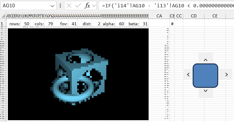
The resulting Excel file is a workbook consisting of more than 6 sheets:

1. The first sheet, R, contains everything needed by the end user: cells with parameters rows, cols, fov, alpha, beta, dist, as well as result cells colored according to a black-and-white scale.
2. The N sheet pre-computes values of $$\frac{1}{\parallel \mathrm{raydir}(s,t)\parallel }$$ .
3. The X, Y, and Z sheets calculate the coordinates X, Y, Z of the vectors raydir(s, t) and $$\frac{\mathrm{raydir}(s,t)}{\parallel \mathrm{raydir}(s,t)\parallel }$$ .
4. The sheets i1, i2,… contain iterations of the Ray Marching algorithm for each pixel.

All sheets follow the same pattern:

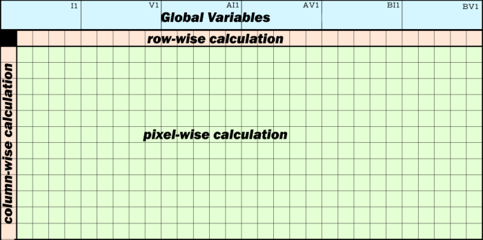
1. The first row contains 1-6 "global" variables (blue). They can be used across all sheets.
2. Most of the sheet is occupied by pixel computations (green). This is a rectangle of size rows\times cols. In the tables at the end of the article, these cells are marked as **
3. The X, Y, and Z sheets also use intermediate computations by rows and columns (orange). The second row and first column are reserved for these. In the tables at the end of the article, these cells are marked A* and *2. The idea is that to store values of raydir(s, t) for all pixels, it is not necessary to add three more sheets (one for each coordinate) since its computation formula is broken down into the sum of two components:

$$\mathrm{raydir}(s,t)=\underset{\text{by columns}}{\left(\begin{array}{c}\mathrm{x0}\\ \mathrm{y0}\\ \mathrm{z0}\end{array}\right)+s\cdot \left(\begin{array}{c}\mathrm{ux}\\ \mathrm{uy}\\ \mathrm{uz}\end{array}\right)}+\underset{\text{by rows}}{t\cdot \left(\begin{array}{c}\mathrm{vx}\\ \mathrm{vy}\\ \mathrm{vz}\end{array}\right)}$$

Thus, we precompute the first term by columns and the second by rows, and when we need to obtain the value of raydir(s, t), we sum the value of the cell for row s and column t.

I1

V1

AI1

AV1

BI1

BV1

**

I1

**

I1

V1

AI1

AV1

A*

*2

**

I1

V1

AI1

A*

**

I1

V1

AI1

AV1

A*

*2

**

I1

**

**

Notes:

Since Excel performs calculations in radians, the arguments of all trigonometric functions are multiplied by $$\frac{\pi }{180}$$ (in Excel, this is done using the RADIANS function). To avoid confusing the formulas, I removed these multiplications in the tables above. They are all included in the example files:

Download the example of creating 3D graphics in Excel

Download the template for generating a 3D teapot model in Excel

Download the 3D game using Excel formulas

In conclusion, it can be asserted that with Excel formulas, one can create a simple 3D engine or even a 3D game in Excel. The greatest benefit of these examples is the ease of learning the basic principles of 3D graphics creation through simple Excel formulas. Once these principles are mastered, they can be transferred to any programming language for expanded capabilities and significant results in development. The entry barrier for mastering Excel formulas is always lower than for any programming language. I recommend starting programming education using Excel formulas and functions. They are easy to learn, and the principles of Excel functions are very similar to programming languages.