How to learn Excel on your own

Microsoft Excel is an extremely useful program to be applied in many spheres. It is a ready-made spreadsheet with such features as auto-fill, prompt calculation and computation, construction of graphs and diagrams, generating reports and evaluations, etc.

Spreadsheet processor tools can significantly facilitate the work of various professionals. The information presented below comprises Excel essentials for complete beginners. Study this article to gain basic skills necessary for starting any operation in Excel.



How to work in Excel tutorial

Excel consists of sheets. Sheet is a work area in the window. Its components are as follows:

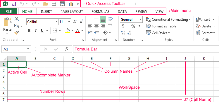
To add a value to the cell, left-click on it. Type the text or numbers. Press Enter.

Values can be numeric, text, currency or percentage-related, etc. To set up / change the format right-click the cell and select «Format cell». Alternatively, press the hot keys combination CTRL+1.

For number formats you can assign quantity of decimal places.

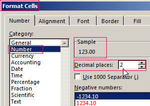
Note. To set up the numeric format for a cell quickly press the hot keys combination CTRL+SHIFT+1.

For «Date» and «Time» formats Excel offers several variants of value representation.

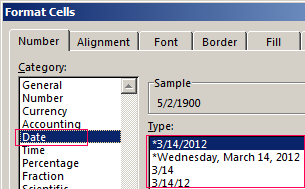
Let’s edit the cell value:

1. Left-click the cell with a word and type a number. Press ENTER. The word is deleted and the number remains.
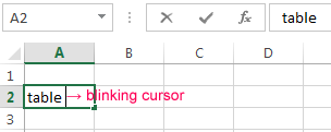
2. For the previous value to remain but to be changed, double click the cell. The cursor will start blinking. Change the value: delete part of the text, add what you need.

3. The value can also be edited through the formula bar. Highlight the cell, place the cursor in the formula bar, edit the text (number), and press Enter.

To delete the cell value, use the Delete key.

To move the cell with a value, highlight it, select the scissors icon («Cut»). Alternatively, press CTRL+X combination. A dashed line will appear around the cell. The highlighted text will remain in the clipboard.

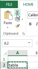
Put the cursor in another work area place and click on «Paste» or press CTRL+V combination.

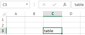
In the similar way you can move several cells simultaneously to the same sheet, to another sheet or to another workbook.

To move several cells you need to highlight them:

1. Place the cursor in the top leftmost cell.
2. Press Shift, and keeping it pressed highlight the whole range with the help of arrow keys.

To highlight a column, click its name (Latin letter). To highlight a row, click its number.

To change the size of rows or columns, move cell borders (in this case the cursor looks like a cross, whose horizontal line has arrows at the ends).

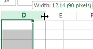
To fit the value in the cell, the column can be expanded automatically by double clicking on the right border.

To preserve the column width but increase the row height click «Wrap Text» on the button ribbon.

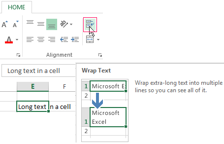
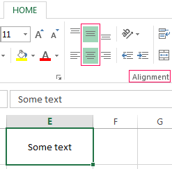
To make it look better, move a little the border of column E and align the text to the center against the vertical and horizontal directions.

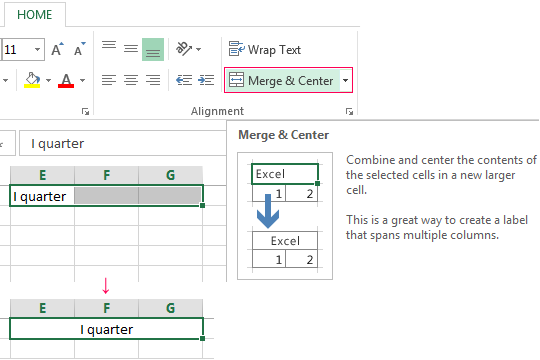
Merge several cells: highlight them and click «Merge & Center».

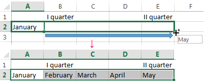
Excel has an auto-fill function. Type the word «January» in A2. The program recognizes the date format and adds other months automatically.

Grab the bottom right corner of the cell with «January» value and drag it along the row.

Let’s test the auto-fill function on numerical values. Type «1» in cell A3 and «2» in cell F4. Highlight two cells, grab the auto-fill marker and drag it downwards.

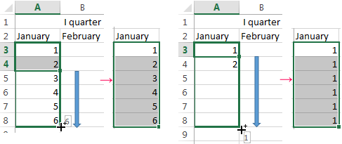
If we highlight only one cell with a number and drag it downwards, this number will “multiply".

To copy the column to the adjacent one, highlight it, grab the auto-fill marker and drag it downwards.

In the similar way, you can copy rows.

Delete the column: highlight it, right-click and select «Delete». Alternatively, press the hot keys combination: CTRL+"-"(minus).

To insert a column, highlight the adjacent right one (a column is always inserted to the right side), right-click, select «Paste», then - «Column». Alternatively, use the combination CTRL+SHIFT+"=".

To insert a row, highlight the adjacent lower one. Use key combination SHIFT+SPACEBAR to highlight a row. Right-click, select «Insert», then «Row» (CTRL+SHIFT+"=") (a row is always inserted above).



How to use Excel: formulas and functions for newbies

For the program to accept the information typed in the cell as a formula, use «=» character. For example, = (2+3)*5. As soon as you press «ВВОД», Excel calculates the result.

The sequence of calculation is the same as in Mathematics.

A formula may contain not only numerical values, but also references to the cells with values. For example, =(A1+B1)*5, where А1 and В1 are references to the cells.

To copy the formula to other cells, you need to grab the auto-fill marker in the cell with the formula and drag it downwards (to the side if you copy to row cells).

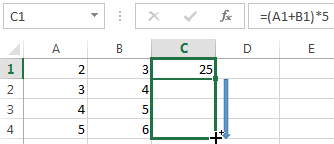
When you copy formula with relative references to cells, Excel changes constants depending on the current cell (column) address.

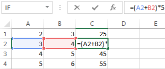
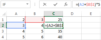
To make the reference absolute (permanent) and ban changes against a new address, a dollar symbol ($) is used.

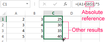
In each cell of column C the second component in brackets is 3 (the reference to B1 is permanent and unchangeable).

Imbedded functions significantly expand program’s functionality. To insert a function you need to press fx button or the key combination SHIFT+F3. The window will open:

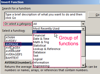
To avoid scrolling a long list of functions you need to choose the category.

When the function is chosen, click OK. «Function Arguments» window will open.

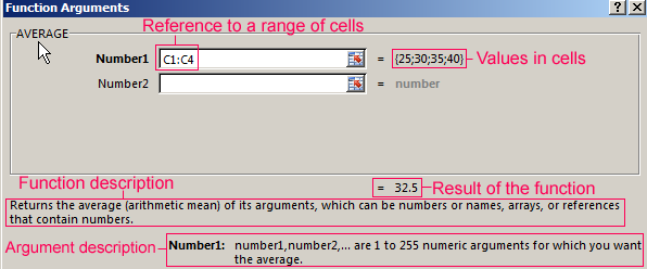
Functions recognize both numerical values and references to cells. To insert a reference in the argument field, click the cell.

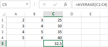
Excel also recognizes another way of entering function. Type «=» symbol in the cell and start entering the function name. After the first characters a list of possible variants will appear. If you place the cursor on one of them, a prompt will appear.

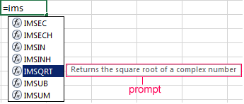
If you double click the required function, the order of argument entering will become available. To finish argument entering close the bracket and press Enter.

Function argument = IMSQRT() – reference to A1.

Enter – the program has found the square root of 40.