How to make a Crossword Puzzle with Excel Functions for Clue
Everyone likes to solve crosswords. This is an extremely useful thing that will come in handy in different areas of activity: to attract users to the resource, to check and consolidate knowledge during teaching, etc.
Excel spreadsheets allow users to “automatize” solving crossword puzzles: they can immediately see the results of the solution. Let’s create them using standard functions.
How to make an interactive crossword in Excel
The standard Excel sheet is a set of rectangular cells that are not quite suitable for drawing crossword puzzles. So first you need to make them square.
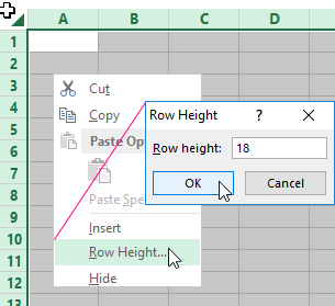
Select all the cells by pressing Ctrl + A. Right-click anywhere and select «Row Height». Set the value to 18.
Change the width of the column by another way: grab the right edge of any cell and move it to the left side, setting the value to 3.
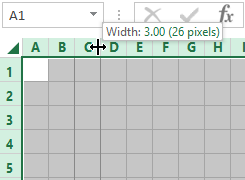
At the same time, the width of all columns of the worksheet is changed.
Begin drawing the grid of the crossword puzzle. Select the required quantity of cells. Set all the boundaries in «Font» group.
By the same principle, draw the entire crossword. Don’t forget to put numbers of questions / answers.

Make up questions for the crossword puzzle. Write them to the right of the grid.
Value on a spreadsheet crossword clue
How to Make a Crossword with Checking in Excel: Create an Auxiliary Table with Answers on a New Worksheet:
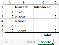
In «Introduced:» column, the answers entered in the crossword by a user will be displayed. Column "?" represents matches. Cell V8 displays the number of correct answers.
Now glue the individual letters in the crossword into whole words by using «CONCATENATE» function. Enter formulas in «Introduced:» column’s cells:

A user can enter both lowercase and uppercase letters. As a result, some problems arise. To avoid them, use «LOWER» function. Place it in all cells before «CONCATENATE» function.
Excel function crossword clue for questions:
- In cell C2:
- In C3:
- In C4:
- In C5:
- In C6:
The function converts uppercase letters to lowercase ones.
If a user enters a correct answer, figure 1 will appear in column range D2:D6. In case of an incorrect answer, 0 will appear. In cell D2 do it by using «=IF()» function: =IF(B2=C2,1,0). For calculating the number of correct answers, =SUM(D2:D6) function is used in cell D7.
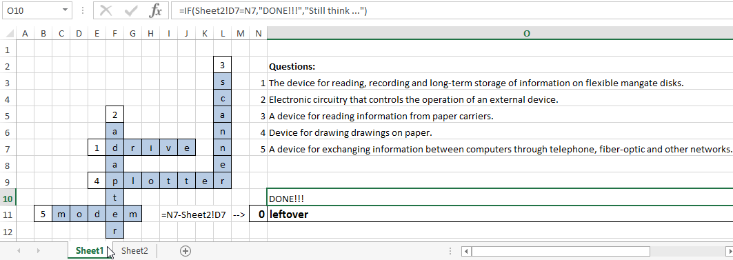
The number of all correct answers is 5 in cell Sheet1!N7. If "5" appears in «Total» cell Sheet2!D7, it means that a user coped with solving the crossword. The message “DONE!!!” (for example) is displayed on the screen.
If there is another number in «Total» cell, “Still think …” is displayed.
Implement the task using «IF» function in cell O10 on Sheet1:
Let’s show a user how many answers are left to guess. The total number questions is 5 (in cell Sheet1!N7) . Hence, the formula will be as follows in cell N11 on Sheet1:
=N7-Sheet2!D7
Where Sheet2!D7 – is the number of correct answers from the auxiliary table.
To check the functionality of the formulas, enter all the answers into the grid of the crossword. You’ll get the following result:
Hide the correct answers from a user. Remove them from the crossword grid on the second worksheet. Select the rows of the auxiliary table. Go to «DATA» tab - «Outline» group. Use «Group» tool.
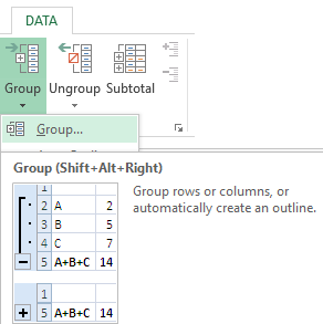
In the opened window, select the check box in front of «Rows» entry.
The structure icons and the minus symbol will appear in the left field of the worksheet.
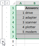
Click on "-" icon. The auxiliary table data will become invisible.
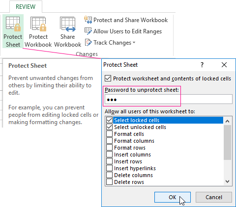
Next, go to «REVIEW» tab. In «Changes» group, find «Protect Sheet» button. Assign a password in the opened window. Now an unauthorized person (who doesn’t know the password) will not be able to open the auxiliary table and see the answers.
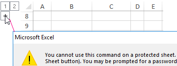
If a user tries to open the answers, the program will show the following warning: "You cannot use this command on a protected sheet...".
The basic work on creating the crossword puzzle is over. You can beautifully finalize the worksheet, add a name, change the fill color of the grid, brighten the borders of cells, etc.
