CONCATENATE function and Opposite of concatenate in Excel
The function CONCATENATE is used to combine values (textual and numerical) from different cells into one. Its analog is & (ampersand). The sign copes with the simplest tasks. But it is not suitable to combine a lot of rows.
Syntax of the concatenate function
The function is part of the "text" group. Syntax: (txt1; txt2; ...). You can include up to 255 text strings. The first argument "text 1" is mandatory. Any arguments can be specified as text, numbers or cell references.
General rules for using the CONCATENATE function:
- Use a semicolon to separate arguments. Skipping or using other characters will cause an error to be displayed.
- The text arguments must be enclosed in quotes. Otherwise, an error appears in the form of the inscription # NAME? Numbers and cell references are not necessary.
- You need to add spaces to the formula with the function in order for the united elements in the result line to be displayed with "space". Using double quotes with a space inside (" ") or with "space" after the text argument ("Ivanov "; ...).
How to use the concatenate function in Excel?
Let's begin with the simplest examples. Data to be merged:

We put the cursor in cell E2 and call the formula wizard (button fx). In the category "Text" we find the name CONCATENATE. Alternatively, select: «FORMULAS»-«Text»-«CONCATENATE». Arguments are references to cells A2, B2, C2 and spaces:
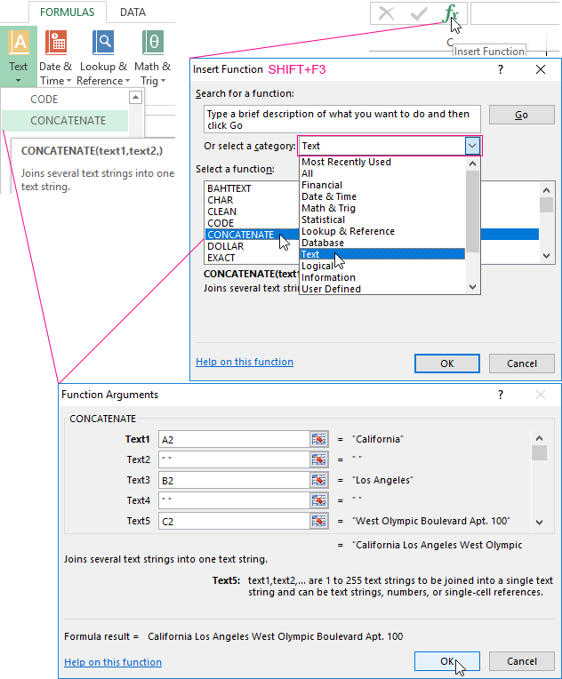
The result of combining values in cells:

The same result is obtained with the help of an ampersand:

One of the arguments is text. Formula: Result:

The CONCATENATE function in Excel will do more complex tasks. Examples:
- Connect the text with the date. The data is in separate cells. The "Date" column is set to "Date" format. The date will be displayed in numerical format if you use only the CONCATENATE function. Therefore, we add the function TEXT to format the numbers. Formula: The second argument of the TEXT function is the date format. Result:
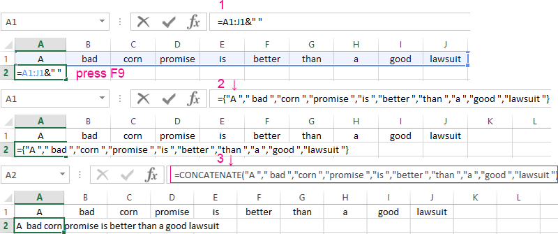
- We connect many cells in a row at once. It will be long and inefficient if you write a formula with the CONCATENATE function. We use a little trick. Here is our line with the values in the separate cells. We put the sign "equal" in cell H1. Select the range with the values A1: J1. Enter ampersand & and space " ". Push F9 button. The array formula appears in the formula bar. We put the cursor in the formula line after the "equal" sign. Write word CONCATENATE. Curly brackets are replaced by round brackets and then press ENTER. We get the desired result.
- We connect values using slash ("-", "&", etc.). The formula will look like this: = CONCATENATE( a reference to cell 1; "/"; reference to cell 2).


Opposite of CONCATENATE in Excel
There is no standard function that would separate the values of one cell. You can use other functions to perform a number of similar tasks:
- LEFT (displays the specified part of the characters from the beginning of the line);
- RIGHT (displays the specified part of the characters from the end of the line);
- MID (displays the specified part of the characters starting at the specified position) and others.
Examples Inverse CONCATENATE function:
- We extract the first word from the string by applying the LEFT function - first opposite of concatenation in Excel. Arguments are "text" ( a reference to the string with the desired value), "quantity of characters" (the character quantity is to be extracted).
- Let's extract the last word from the line using the RIGHT function. The syntax is similar (as in the previous example). Only the quantity of characters is counted from the end.
- The main opposite of concatenation in Excel is MID. We extract a surname (the second word) from the entry in the line with the help of the MID function. Arguments are "text" ( a reference to a string), "initial position" (the symbol number from which the program will start counting the character quantity; " quantity of signs". In the example: E2 - "text", after the 9th symbol, the formula will return 8 characters.


More complex formulas are used and user functions are compiled to perform more complex tasks.
Example of Practical Application of the CONCATENATE Function
The CONCATENATE function is very effective and is often used in combination with the INDEX and MATCH functions as a formula for searching and retrieving data from a table based on multiple criteria.
Using CONCATENATE with INDEX and MATCH for Multiple Criteria
For example, we have a table with monthly values for 2 years. The first column is "Years," the second column is "Months," and the third column is "Sum Values":
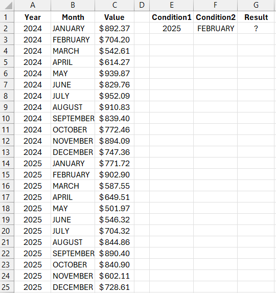
We need to get the sum value for a specific year and a specific month. Therefore, the formula must handle two criteria: the year number and the month name.
To easily understand the principle of how the data extraction formula works, let's break the process into two steps: find the value and extract it. We'll extract it using the INDEX function. In its first argument, we'll specify the cell range containing the values in the third column of the source table, C2:C25. For the second argument of the INDEX function, we need to specify the row number of the table. We'll search using the MATCH function based on two criteria simultaneously across the first two columns of the table.
If you look at the values in the first two columns of the table, you can easily identify each value from the two columns in one row, forming a unique ID code for each row. For example, for the first row, the code is 2024JANUARY, for the second 2024FEBRUARY, and so on…
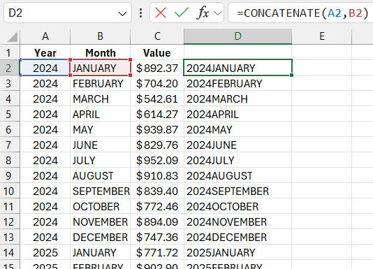
Thus, we can use the CONCATENATE function in the arguments of the MATCH function to search for the row number based on two criteria. The Excel formula:
=IF(E$3,INDEX(Data!$C$2:$E$73,MATCH(CONCATENATE($A$25,$D7),CONCATENATE(Data!$A$2:$A$73,Data!$B$2:$B$73),0),E$4),NA())
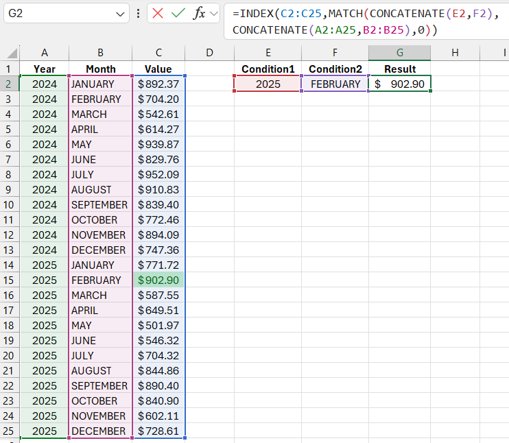
It is important to note that if we use the CONCATENATE function in the first argument of the MATCH function, it must also be used in the second argument, specifying references to the ranges of the columns being searched.
When preparing and processing data for visualization in Excel, it is often necessary to search and retrieve data from tables of source values. For developing interactive dashboards, data retrieval must be implemented based on multiple criteria. For this, we use a formula with the CONCATENATE function. An example of such a dashboard:

Download an example of using the CONCATENATE function for a dashboard in Excel 
See examples of formulas on different sheets of the template.
