Examples of functions COUNT, COUNTBLANK and COUNTIF in Excel
The numbers of numbers in the Excel spreadsheet can be quickly figured out using the COUNT function. Ignoring textual format, it takes into account only numeric values.
Where is the COUNT function used and how does it work?
Often, for the analysis of tabular data it is not necessary to perform any mathematical operations with numbers. It is enough to clarify the number of indicators. It is for such a case that this simple COUNT function is useful.
The function argument can be:
- any values copied and put in place of the argument;
- single cell or whole table area;
- formulas and functions.
The syntax of the function is as follows:
=COUNT(value1,[value2],...)
All versions of Excel, starting from 2007, can take up to 255 arguments when calculating the result of this formula. Only the first one is required. There is a difference in how the value is taken into account if it is stored in a cell or entered in the number of arguments.
- Numbers, dates, and times are always counted by the COUNT function.
- Text and errors are never taken into account.
- Logical values and the textual representation of a number are not taken into account if it is stored in a cell. If the same elements are entered into the formula as an argument, they will be taken into account.
To understand this feature you need to consider visually with specific examples.
Example of using the COUNT function in Excel
Example 1. Some values are entered in the table. Among them is a text, numeric expressions and a number enclosed in quotation marks "22". That is what Excel considers the text value in the cell.
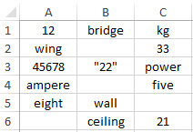
Let's write the formula, it will take into account the contents of the array of cells, and will look like this:
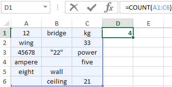
After entering the formula by pressing the Enter key, the number 4 will appear. These are the numbers entered in the cells using numbers that are not enclosed in quotes.
Now we will enter another function in the cell below D2. In it all tabular elements will be registered in the form of arguments. It will look like this:
=COUNT(12,bridge,kg,wing,33,45678,"22",power,ampere,five, eight,wall,ceiling,21)

Entering the formula, we get the value 5.
Different results of the function are explained by the fact that one number (“22”) is perceived by the program as text if it is in a cell, and as a number if it is written in the number of function arguments.
Example of using COUNTA and COUNTBLANK functions in Excel
You can quickly determine the number of filled or empty cells in a given area of the table. To perform these operations, functions with the name COUNTA and COUNTBLANK are used. For clarity of this opportunity, it is necessary to consider an example.
Example 2. In the table entered different values. There are no patterns among them. There are empty and filled cells.
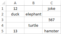
You can enter a function anywhere in the table. To determine the filled cells in the A1:C5 range, you need to prescribe the following formula:
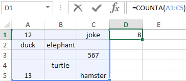
Entering it through Enter will give the result of 8. It is the number of filled cells in the designated area.
To find out the number of empty cells, you need to enter the function COUNTBLANK:
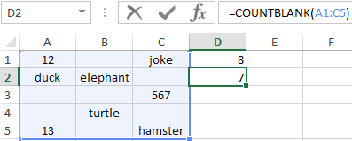
The introduction of the formula will show the result 7. This is the number of empty cells in the table.
Example of using the function COUNTIF with the condition
This type of function COUNT is very often used. Using a given formula, you can find out the number of cells with specified parameters. The function has the name COUNTIF. It can take into account such arguments.
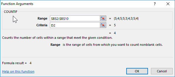
- Range. The table area in which certain elements will be searched.
- Criterion. A sign that is searched in a given area.
The syntax is:
The function can show the number of cells with the specified text. For this argument is quoted. It does not take into account the text register. There can be no spaces in the formula syntax.
Both arguments are required for reference. For clarity, consider the following example.
Example 3. There is a statement with the names of students and marks for the exam. The table has 2 columns and 10 cells. It is necessary to determine how many students received an excellent grade of 5 (according to a five-point grading system), and which 4, then 3 and 2.
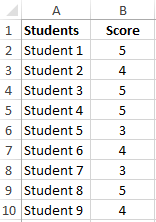
To determine the number of honors you need to analyze the contents of the cells of the second column. In a separate table you need to use a simple function of counting the number of numerical values with the condition COUNTIF.
After pressing the Enter key on the keyboard, the result will be obtained:
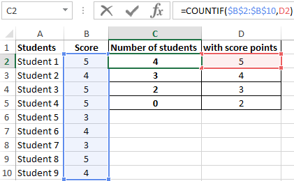
- 4 honors;
- 3 students with a score of 4 points;
- 2 students with score 3 points;
- not Losers.
Download examples COUNT COUNTBLANK COUNTIF in Excel
So, in just a few seconds, you can get data on extensive and complex tables.
