What does SUMPRODUCT function do examples of its using
SUMPRODUCT in Excel – is the favorite function of accountants, because it is most commonly used for the calculation of wages. Although it happens, it is useful in many other spheres.
You can guess by it name, that the team is responsible for the summation of compositions. The compositions in this case are considered either ranges or whole arrays.
The syntax function SUMPRODUCT
The arguments of the function SUMPRODUCT are arrays, that is to say the preset ranges. There can be as many as you like. Listing them through a semicolon, we set the number of arrays, which must first be multiplied, and then summed. The only condition is that the arrays must be equal in length and of the same type (that is, either all horizontal or all vertical ones).
The simplest example of using the function
To make it clear how and what the team believes, we consider the simple example. We have the table with the specified lengths and widths of the rectangles. We need to calculate the sum of the areas of all the rectangles. If you do not use this function, you will have to perform intermediate actions and calculate the area of each rectangle, and only then the sum - as we have done.
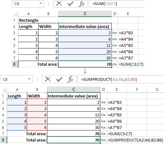
Pay attention that we did not need an array with subtotals. In the arguments of the function, we used only arrays of length and width, and the function automatically multiplied and summed them, yielding the same result = is 70.
SUMPRODUCT with the condition
The function SUMPRODUCT in its natural form is almost not used, because the calculation of the amount of works can rarely be useful in production. One of the popular applications of the SUMPRODUCT formula – is to output values that satisfying by specified conditions.
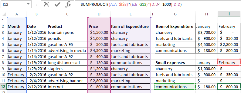
Let's consider the example. We have the cost table for a small company for one month. It is necessary to calculate the total amount spent for January and February for all items of expenditure.
For calculating of the costs for the chancellery in January-month, we use our function and specify in the beginning two conditions. Each of them we enclose in parentheses, and between conditions need to put the «asterisk» sign, meaning the «and» union. We get the following command syntax:
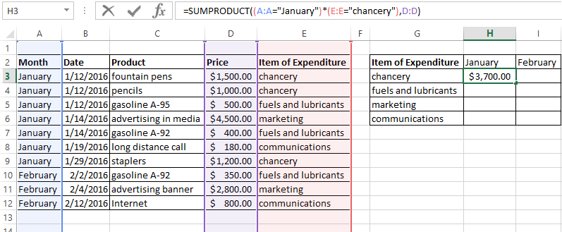
- A:A = «January») - the first condition;
- E:E = «chancery» - the second condition;
- D:D – is the array, from which the total amount is displayed.
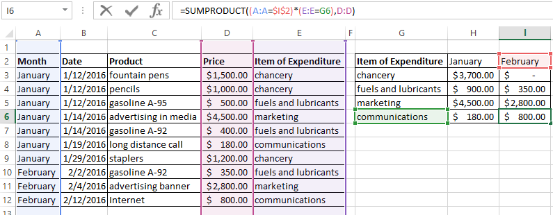
As a result, it turned out that in January 3,700 dollars were spent for office supplies. We will extend the formula to the remaining lines and replace in each of them the conditions (replacing the month or the item of expenditure).
The comparison in SUMPRODUCT
One of the conditions when using the SUMPRODUCT command can be a comparison. Let's consider at once on the example and suppose that we need to calculate not just all office expenses for January, but only those that were less than 1000 dollars (let's call them «the small expenses»). We prescribe to the function with the same arguments, but in addition we place the comparison operator. In this case, it looks like D:D >= 1000. The command issues to the following response: 1000.
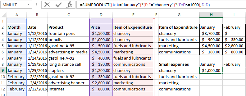
And indeed, this is the thousand that was spent in January on the pencils. We also set the comparison condition, and when the value was automatically returned and the function gave us such the response.
Download all examples SUMPRODUCT in Excel.
We extend the formula to the remaining cells, partially replacing to the information. We discover how much money was spent in January and February for small expenses for each cost item.

Data Visualization Charts for Interactive Report Creation in Excel.
Dashboard Templates