Difference between VLOOKUP and HLOOKUP with examples

The functions VLOOKUP and HLOOKUP among Excel users are very popular. The first function is used for vertical analysis, comparison. That is, it is used when the information is concentrated in columns.

HLOOKUP, respectively, is used for horizontal analysis. Inasmuch as there are rarely more rows in tables than columns, this function is rarely called.

The syntax of the VLOOKUP and HLOOKUP functions

The functions have 4 arguments:

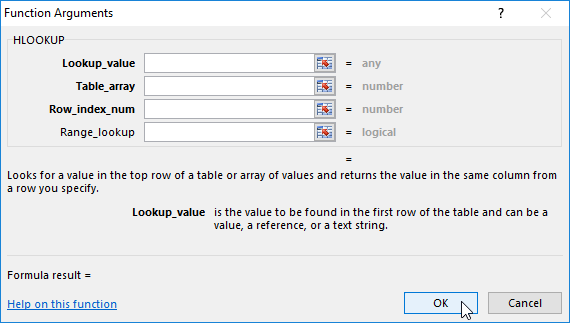
Lookup value: WHAT we are looking for – the desired parameter (numbers and / or text) or a reference to the cell with the desired value;
Table array: WHERE we are looking for – an array of data where the search will be performed (for VLOOKUP – the searching of the value is carried out in the FIRST column of the table, for the HLOOKUP – from the FIRST line);
Row index number: The NUMBER of the column / row – where exactly the corresponding value is returned (1 – from the first column or the first line, 2 – from the second one, etc.).
Range lookup: The INTERVAL VIEW – the exact or approximate value should be found by the function (FALSE / 0 – the exact value, TRUE / 1 / not specified – the approximate value).

Attention! If the values in the range are sorted in ascending order (or alphabetically), we specify TRUE / 1. Otherwise – there is FALSE / 0.

How to use the VLOOKUP function in Excel: examples

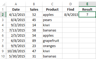
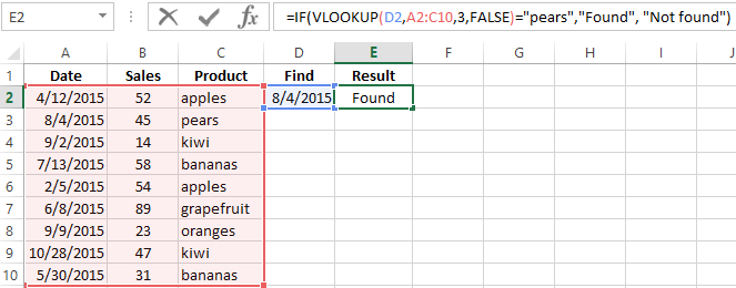
For the educational purposes, let's take the table with the data:

Formula	Description
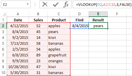
=VLOOKUP(D2,A2:C10,3,FALSE)	The function searches for the value of the cell F5 in the range A2:C10 and returns the value of the cell F5, that was found in the column 3, the exact match.

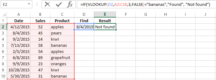
=IF(VLOOKUP(D2,A$2:C$10,3,FALSE)="bananas","Found", "Not found")	We need to find out whether bananas were sold 04. 08. 15. If bananas sold, the word «Found» appears in the corresponding cell. If bananas weren`t sold – «Not found».

=IF(VLOOKUP(D2,A2:C10,3,FALSE)="pears","Found", "Not found")	If the «bananas» are changed to «pears», the result will be «Found»

=IFERROR(VLOOKUP(D2,A2:C10,3,FALSE),0)	When the VLOOKUP function can not find a value, it gives an error message # N/A. To avoid this, we use the function IFERROR.
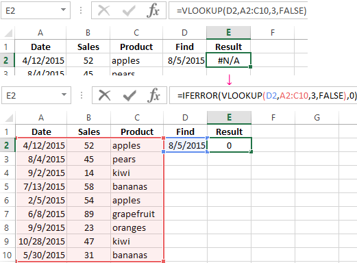We will find out whether there were sales 08.05.15
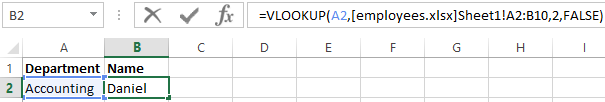
=VLOOKUP(A2,[employees.xlsx]Sheet1!A2:B10,2,FALSE)	If it`s necessary to implement for the search value in the another Excel workbook, then when filling out the «table» argument, we go to another workbook and select the desired range with the data.
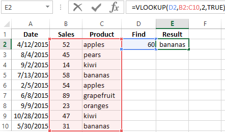
We wanted to know who worked 06. 08.15.
=VLOOKUP(D2,B2:C10,2,TRUE)	The searching of the approximate value.

It is important:

The VLOOKUP function always searches for data in the leftmost column of the table with values.
The register is not taken into account: small and large letters for Excel are the same.
If the sought after is less than the minimum value in the array, the program will return the error # N/D.
If you set the column number to 0, the function will show #VALUE. If the third argument is greater than the number of columns in the table - #REFERENCE.
To copy the correct array, we apply to the absolute references (F4 key).

How to use by the HLOOKUP function in Excel: examples

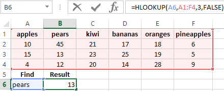
For educational purposes, let`s take the following table:

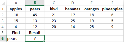
Formula	Description
=HLOOKUP(A6,A1:F4,3,FALSE)	Find the value of the cell \|16 and return of the value from the third row of the same column.

The application of HLOOKUP in practice is limited, inasmuch as the horizontal representation of the information is used very rarely.

The symbols of substitution in VLOOKUP and HLOOKUP functions

It happens that the user does not remember the exact name. By specifying the desired value, he can apply the wildcard characters:

«?» – replaces any character in text or digital information;
«*» – for replacing any sequence of characters.

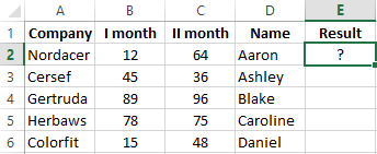
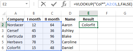
Let`s find the text that begins or ends with a certain set of characters. For example we need to find the name of the company. We forgot it, but remember that it starts with Kol. The problem will be solved by the following formula:

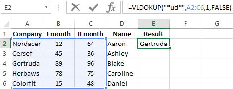
We need to find the name of the company that ends with – «uda». The following formula will help:

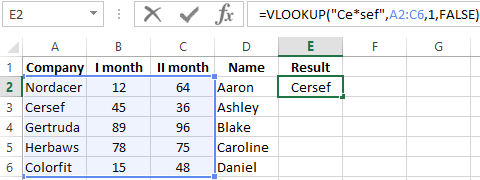
Let`s find a company which name begins with «Ce» and ends with «sef». The formula of the VLOOKUP will look like this:

When the problems with memory are eliminated, you can work with data using all of the same functions.

How to compare sheets with the helping of VLOOKUP and HLOOKUP?

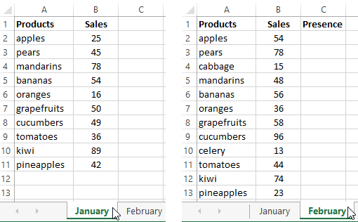
We have data about sales for January and February. These tables need to be compared using the formulas VLOOKUP and HLOOKUP. For clarity, we'll put them in one sheet for now, but we will work in conditions when the ranges are in different sheets.

How can I compare sheets using VLOOKUP in Excel?

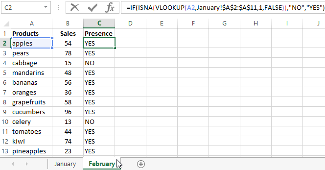
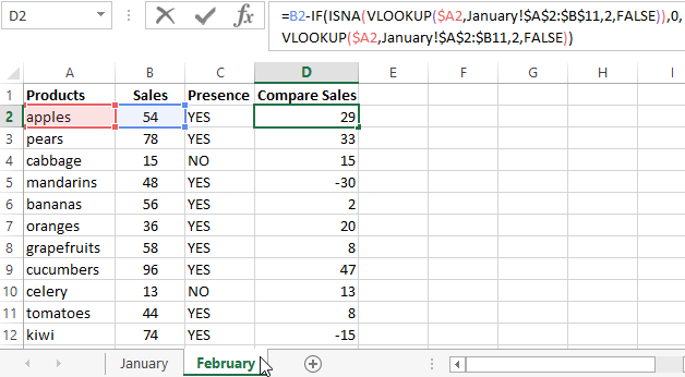
Let`s solve the problem 1: we compare the names of goods in January and February. Inasmuch as there are more of them in February, we will enter the formula on the «February» sheet.

Let`s solve the problem 2: we compare the sales by positions in January and February. We use the following formula:

How can I compare sheets with HLOOKUP in Excel?

To demonstrate the action of the HLOOKUP function, we take two «horizontal» tables, located on different sheets.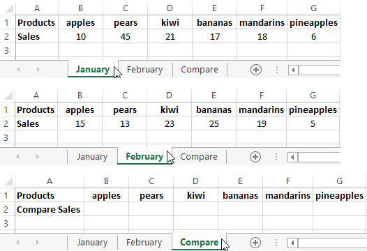 demonstrate.

The task – is to compare sales by positions for January and February.

We create the new «Compare» sheet. This is not the obligatory condition. You can compare the data and display the difference on any sheet («January» or «February»).

The formula:

The result:

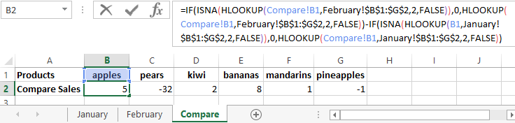
Let analyze the parts of the formula:

«Half» up to the sign «-»:

=IF(ISNA(HLOOKUP(Compare!B1,February!$B$1:$G$2,2,FALSE)),0,HLOOKUP(
Compare!B1,February!$B$1:$G$2,2,FALSE))-

The desired value – is the first cell in the table for comparison. The analyzed range – is the table with sales for February. The HLOOKUP function «takes» data from the second line in «accurate» reproduction.

After the «-» sign:

-IF(ISNA(HLOOKUP(B1,January!
$B$1:$G$2,2,FALSE)),0,HLOOKUP(Compare!B1,January!$B$1:$G$2,2,FALSE))

There are all the same in addition to the range. Here we take the table with sales for January.

Download example functions VLOOKUP and HLOOKUP

When we enter a formula, Excel prompts about: what the argument you need to enter now.