How to find the arithmetic mean in Excel?
There are many functions in order to find the average in Excel (although it does not matter what kind of value it is: numerical, textual, percentage or other). And each of them has its own peculiarities and advantages. After all, certain conditions can be put in this task.
For example, the average in Excel is counting using statistical functions. You can also manually enter your own formula. Consider the various options.
How to find the arithmetic mean?
It is necessary to add all the numbers in the set and divide the sum by the number in order to find the arithmetic mean. For example, the student's marks in computer science: 3, 4, 3, 5, 5. The average rating is 4 for a quarter. We found the arithmetic mean using the formula: =(3 + 4 + 3 + 5 + 5) / 5.
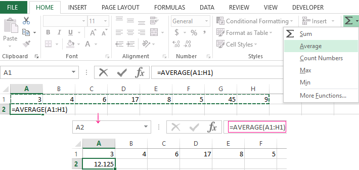
How can you quickly do this with Excel functions? Take for example a number of random numbers in a row:

- We put the cursor in cell A2 (under a set of numbers). In the menu – «HOME»-«Editing»-«AutoSum»-«Average» button. A formula appears after clicking in the active cell. Select the range: A1: H1 and press ENTER.
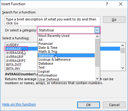
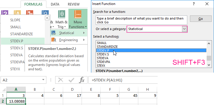
- The second method is based on the same principle of finding the arithmetic mean. But we will call the function AVERAGE differently. Using the function wizard (use fx button or key combination SHIFT + F3).
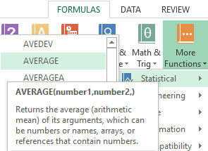
- The third way to call the AVERAGE function from the panel: «FORMULAS»-«More Function»-«Statistical»-«AVERAGE».
Or you can make cell to be active and just manually enter the formula: =AVERAGE(A1:A8).
Now let's see what the AVERAGE function be able to:
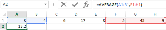
Let us find the arithmetic mean of the first two and three last numbers. Formula: =AVERAGE(A1:B1,F1:H1).
Average value by condition
A numerical criterion or a textual criterion can be the condition for finding the arithmetic mean. We will use the function: = AVERAGEIF().
Find the arithmetic mean for numbers that are greater or equal to 10.
Function:
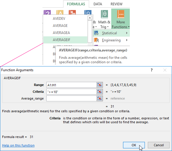
The result of using the function "AVERAGEIF" by the condition ">=10" is next:
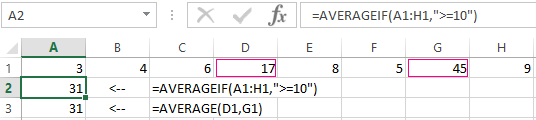
The third argument "Averaging Range" is omitted. Firstly, it is not necessary. Secondly, the range analyzed by the program contains ONLY numeric values. In the cells specified in the first argument, the search will be performed according to the condition specified in the second argument.
Attention! You can specify the search criteria in the cell. And in the formula make a reference to it.
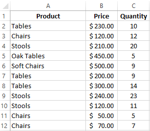
Let's find the average value of numbers by the text criterion. For example, the average sales of goods "Tables".
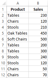
The function will look like this:
Range is a column with the names of goods. Search criteria is a link to a cell with the word "Tables" (you can insert the word "Tables" instead of the A7 link). The averaging range is the cells from which data will be taken to calculate the arithmetic mean.
We get the following value as a result of calculating using the function:
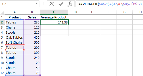
Attention! It is mandatory to point the averaging range for the text criterion (condition).
How to calculate the weighted average price in Excel?
How to calculate the average percentage in Excel? For this purpose, the SUMPRODUCTS and SUM functions are suitable. Table for an example:
How did we know the weighted average price?
Formula:
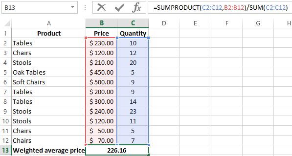
Using the formula =SUMPRODUCT() we learn the total revenue after the realization of the entire quantity of goods. And the =SUM() function sums the goods quantity. We found a weighted average price having divided the total revenue from the sale of goods by the total number of units of the goods. This indicator takes into account the "weight" of each price and its share in the total mass of values.
The standard deviation: the formula in Excel
There is a standard deviation in the entire population and in the sampling. In the first case, this is the square root of the general variance. In the second, this is a square root of the sampling variance.
A dispersion formula is compiled to calculate this statistical indicator. The square root is extracted from it. But in Excel, there is a ready-made function for finding the root-mean-square deviation.
The root-mean-square deviation is related to the scope of the initial data. This is not enough for a figurative representation of the variation of the analyzed range. The coefficient of variation is calculated to obtain the relative level of the data variability.
standard deviation / arithmetic mean
The formula in Excel is as follows:
STDEV.P (range of values) / AVERAGE (range of values).
The coefficient of variation is considered as a percentage. Therefore, set the percentage format in the cell set.

Data Visualization Charts for Interactive Report Creation in Excel.
Dashboard Templates