Changing the format of cells to display data and creating tables
When you fill out Excel worksheets with data, no one will succeed at once, everything is beautiful and correctly filled at the first attempt.
In the process of working with the program, you always need something: modify, edit, delete, copy or move. If the entered incorrect values in a cell, naturally, we want to correct or delete ones. But even such simple task can sometimes create difficulties.
How to set the cell format in Excel?
The contents of each Excel cell consist of three elements:
- The meaning: text, numbers, dates and times, logical content, functions and formulas.
- The formats: the type and color of the borders, the type and color of the fill, the way the values are displayed.
- Comments.
All these three elements are completely independent of each other. You can specify the format of the cell and do not write anything to it, or add a note in an empty and not formatted cell.
How to change the format of cells in Excel?
To change the format of the cells, you should call the corresponding dialog box with the CTRL + 1 (or CTRL + SHIFT + F) key or from the context menu after you right-click the «Cell Format» option.
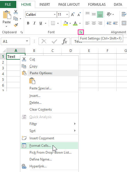
There are 6 tabs in this dialog box:
- A number. Here you specify the way the numeric values are displayed.
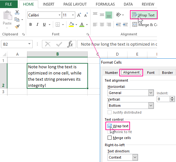
- The alignment. On this tab you can control the position of the text. And the text can be displayed vertically or diagonally from any angle. Also pay attention to the «Display» section. Very often, the function «Wrap Text» is used.
- Font. The specify the style design of fonts, the size and color of the text, plus the modes of modifications.
- The border. Here you define the styles and colors of the borders. The design of all tables is better done right here.
- The fill. The name of the bookmark speaks for itself. Available for formatting colors, patterns and methods of filling (for example, a gradient with a different direction of strokes).
- The protection. Here, the cell protection settings are set, that are activated only after the protection of the whole sheet.
If you did not get the desired result on the first attempt, call this dialog again to fix the cell format in Excel.
What formatting is applicable to cells in Excel?
Each cell always has some format. If there were no changes, then this is the «General» format. It is also a standard Excel format, in which:
- the numbers are aligned on the right side;
- the text is aligned on the left side;
- the font Calibri with the height of 11 points;
- the cell has no borders and background fill.
The Format Removal – is the changing to the standard «General» format (without borders and fills).
It is worth noting that the format of cells, unlike values, can not be deleted with the DELETE key.
To delete the format of cells, select ones and use the «Clear Formats» tool, which is located on the «HOME» tab in the «Editing» section.
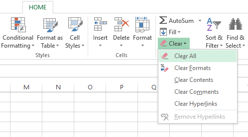
If you want to clear not only the format, but also the values, then select the «Clear All» option from the drop-down list of the tool (eraser).
As you can see, the eraser tool is functionally flexible and allows us to make a choice of what to delete in the cells:
- the content (same as the DELETE key);
- the formats;
- notes;
- the hyperlinks.
The option «Clear all» combines all these functions.
The deleting notes
Note, as well as formats, are not deleted from the cell by pressing the DELETE key. You can delete notes in two ways:
- The eraser tool: the option «Clear notes».
- Click on the cell with the note with the right mouse button, and from the appeared context menu select the option «Delete note».
The notation. The second way is more convenient. If you delete several notes at the same time, you must first select all of its cells.

Data Visualization Charts for Interactive Report Creation in Excel.
Dashboard Templates