How to compare two Excel spreadsheets using 2 columns
We have two tables of orders copied into one worksheet. You need to compare the data of the two tables in Excel and check which positions are in the first table but not in the second one. It makes no sense to manually compare the value of each cell.
Comparing two columns for finding matches in Excel
How can we compare values for two columns in Excel? To solve this task, we recommend using conditional formatting which quickly selects the color of positions that are only in one column. Worksheet with tables:
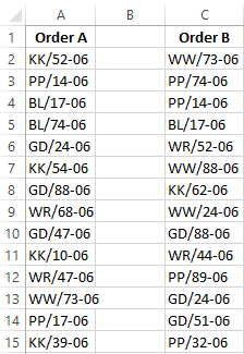
First, you need to name both tables. This makes it easier to understand which cell ranges are compared:
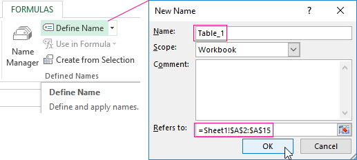
- Select the "FORMULAS" tool - "Defined Names" - "Define Name".
- Enter the value - Table_1 in the appeared window in the field "Name:"
- With the left mouse button click on the input field "Refers to:" and select the range: A2:A15. Then click OK.
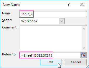
For the second list follow the same steps and just use another name - Table_2. And choose the range C2:C15 respectively.
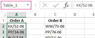
Helpful advice! Range names can be assigned more quickly by using the name field. It is located on the left of the formula row. Just select the ranges of cells, and in the name field enter the appropriate name for the range and press Enter.
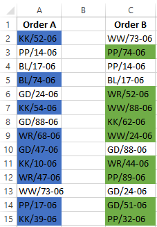
Now let's use conditional formatting to compare two lists in Excel. We need to get the following result:
Positions that are in Table_1, but not in Table_2 will be displayed in green. At the same time, the items in Table 2 which don’t present in Table 1 will be highlighted in blue.
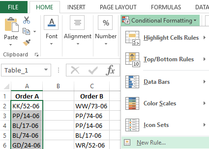
- Select the range of the first table A2:A15 and select the tool: "HOME"-"Conditional Formatting"-"New Rule"-"Use a formula to determine which cells to format:".
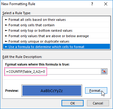
- Enter the formula in the input field:
- Click on the "Format" button and specify a blue color on the "Fill" tab. Click OK in all windows.
- Select the range of the first list C2:C15 and select the tool again – "HOME"-"Conditional Formatting"-"New Rule"-"Use a formula to determine which cells to format:".
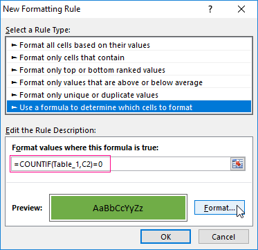
- Enter the formula in the input field:
- Click on the "Format" button and specify the green color on the "Fill" tab. Click OK in all windows.


Principle of comparing the data of two columns in Excel
We used the COUNTIF function when defining conditions for formatting column cells. In this example, this function checks how many times the value of the second argument (for example, A2) occurs in the list of the first argument (for example, Table_2). If the number of times is 0, then the formula returns TRUE. In this case, the cell is assigned a custom format specified in the conditional formatting options. The reference in the second argument is relative, then all the cells of the selected range will be checked in turn (for example, A2: A15).
Download example comparison 2 tables in Excel
The second formula works similarly. The same principle can be applied to various similar tasks. For example, for comparing two prices in Excel and even on different worksheets.
