Merging and splitting data into cells in Excel with formatting
Formatting and editing cells in Excel is a convenient tool for visual presentation of information. These capabilities of the program are priceless.
The importance of optimal demonstration of the data goes without saying. Let's view what we can do with the table cells in Excel. This lesson will teach you some new ways of filling-in and formatting the data in the working sheets.
How to merge cells in Excel without losing data?
Neighboring cells can be merged in vertical or horizontal direction. The result will be one cell occupying two rows or columns simultaneously. The information appears in the center of the merged cell.
Merging cells in Excel step by step:
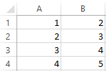
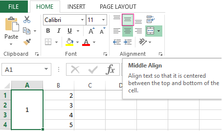
- Let's take a small table with several rows and columns.
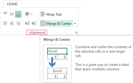
- To merge the cells, use the «Alignment» tool, which can be found on the main tab.
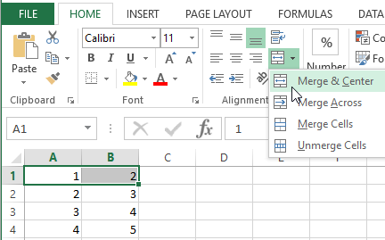
- Select the cells that need to be merged. Click «Merge and Center».
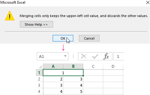
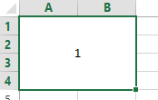
- When the two cells are merged, only the data contained in the top left one is retained. So, if you need to retain all the data, then move it to the top left cell in our case, it's not necessary.
- Likewise, you can merge several cells vertically (a column of data).
- You can even merge a group of neighboring cells in vertical and horizontal directions simultaneously.
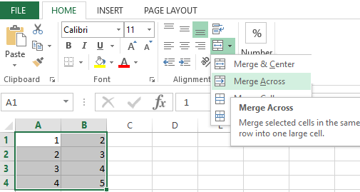
- If you only need to merge the rows in the selected range of values, use the tool «Merge Across».
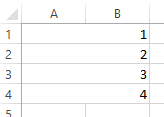
The obtained result will look like this:
If one or more cells in the selected range are being edited, the merging button may be unavailable. You will have to complete the edit first and press «Enter» to leave this mode.
How to split a cell in two in Excel?
Only a merged cell can be split in two. It's not possible to split an individual cell that hasn't been merged. But what if we need a table that looks like this:

Let us have a closer look at this table on the Excel spreadsheet.
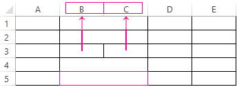
The line does not separate one cells it showcases the border between two. The cells above and below the “split” one are merged in horizontal direction. The first, third and fourth columns in this table consist of one column each. The second consists of two columns.
Thus, in order to split a certain cell in two, you need to merge the neighboring cells. In our examples, the cells above and below. Just don't merge the cell that needs to be split.
How to split a cell diagonally in Excel?
To fulfill this task, you need to perform the following steps:
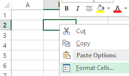
- Right-click on the cell and select the «Format Cells» tool (or use the hot-key combination CTRL+1).
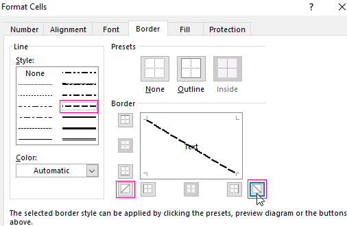
- Go to the «Border» tab and select the diagonal line, its direction, line type, thickness, color.
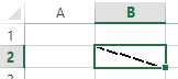
- Click OK.
If you need to draw a diagonal in a large cell, use the «INSERT» tool.
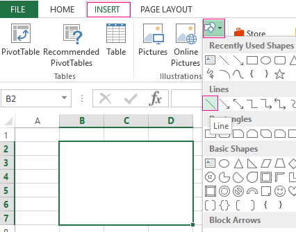
Go to the «Illustrations» tab and select «Recently Used Shapes». The «Line» section.
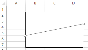
Draw the diagonal line in the needed direction.
How to make the cells uniform in size?
Do the following to make the cells of the same size:
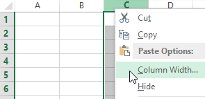
- Select the necessary range containing a certain number. Right-click on the letter above any column. Open the menu «Column Width».
- Enter the needed value of the column width. Chick OK.

The width of the column is indicated in the number of characters of the font Calibri (Body) with height 11 points. Default Column width = 8.43 characters.
To specify the column width in inches in Excel. Do so:
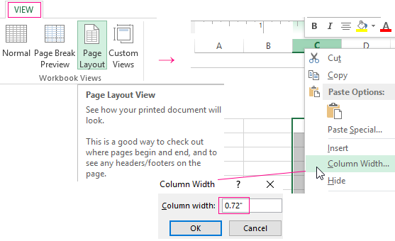
Go to the panel «VIEW». To switch to the «Page Layout». Right-click on the letter above any column. Open the menu «Column Width» in inches. Enter the needed value of the column width. Chick OK.
You can change the width of columns for the entire sheet. To do this, you need to select the whole sheet. Left-click on the intersection of the names of rows and columns (or use the hot-key combination CTRL+A).

Hover the pointer arrow over the names of columns until it looks like a cross. Holding down the left mouse button, drag the boundary to set the desired column width. Now all columns in the spreadsheet are of the same width.
How to split a cell into rows?
Excel allows you to make several rows from one cell. Here we have a few streets listed in a row.
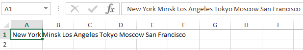
We need to transform them into several rows, so that the name of each street occupies a separate row.
Select the cells. Go to the «Alignment» tab and click the button «Wrap Text».
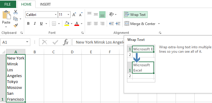
The data from the initial cell will be automatically divided into several rows.
Try your hand at it, experiment. Set the formats that are the most convenient for your readers.

Data Visualization Charts for Interactive Report Creation in Excel.
Dashboard Templates