How to TRANSPOSE a data table in Excel with invert
The concept of «transport» almost does not occur in the work of PC users, but those ones who work with arrays, whether matrices in higher mathematics or the tables in Excel, have to face with this phenomenon necessary.
Transposing a table in Excel is the replacement of columns by rows and vice versa. In other words, it is a turn in two planes: horizontal and vertical ones. There are three ways to transport tables.
The method 1: the special insert
It`s the simplest and universal way. Let's consider at once on an example. We have the table with the price of a certain product per a piece and with certain amount of products. The table cap is located horizontally, and the data is arranged vertically, respectively. The cost is calculated by the formula: price * quantity. For the sake of the clarity, the table header is highlighted in green color.
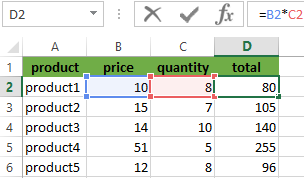
We need to arrange the table`s data horizontally relative to the vertical arrangement of its header.
To transpose the table, we will use the SPECIAL INSERT command. We proceed in these steps:
- We select the entire table and copy it (CTRL + C).
- We put the cursor anywhere in the Excel worksheet and right-click the menu.
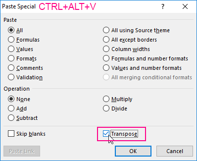
- We click on the command Paste Special (CTRL+ALT+V).
- In the window that appears we put the tick near the TRANSPOSE. The rest we left as is and click OK.
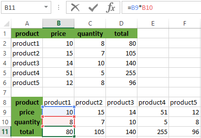
As a result we obtained the same table, but with different arrangement of the rows and the columns. Moreover, we note that cells with the same content are highlighted in green. The value formula was also copied and counted the product of price and quantity, but already with taking into account other cells. Now the table header is located vertically (what is clearly visible due to the green color of the header), and the data are respectively located horizontally.
Similarly, only values can be transposed, without the names of rows and the columns. To do this, you need to select only the array with the values and to do the same with the «Paste Special» command.
The method 2: the TRANSPOSE function in Excel
With the advent of the SPECIAL INSERT, the transposing of the table with using the TRANSPOSE command is almost not used because of the complexity and longer time for the operation. But the TRANSPOSE function is still present in Excel, so we will learn how to use it.
We operate on the stages again:
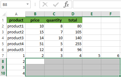
- We select correctly to the range for transposing. In this example of the source table there are 4 columns and 6 rows. Accordingly, we must select the range of the cells in what there will be 6 columns and 4 rows. As it shown on the picture:
- We fill immediately to the active cell so that you do not remove the selected area and enter the following formula: =TRANSPOSE.
- To press CTRL + SHIFT + ENTER. Attention! The function TRANSPOSE() works only in an array. Therefore, after entering it, you must necessarily press the combination of the hotkeys CTRL + SHIFT + ENTER to execute the function in the array, and not just ENTER.

Note that the formula was not copied. When you click on the each cell, you will see that this table has been transposed. In addition, all the original formatting has been lost and you have to align and backlight it again. Also worth paying attention to the fact that the transposed table is tied to the original one. The modified values of the source table are automatically updated in the transposed one.
The method 3: the PivotTable
Those who work closely with Excel know that the PivotTable is multifunctional. And possibility of transpose – is one of its functions. Although it will be look a little bit different than in the previous examples.
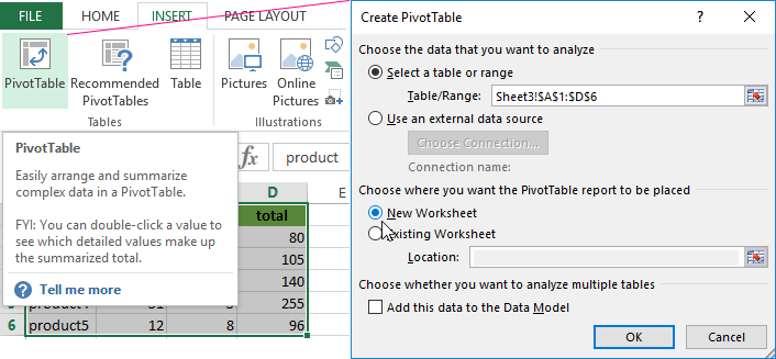
- We will create to the PivotTable. To do this, you need to select the original table and open the INSERT - PivotTable item.
- The place where the summary table will be created, we select the new sheet.
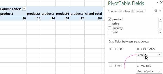
- In the resulting layout of the summary tables, we can select the necessary items and move them to the required fields. We will transfer «product» in the NAMES of COLUMNS, and «the price per piece» in VALUES.
- We obtained the PivotTable for the required field, and the team automatically calculated the grand total.
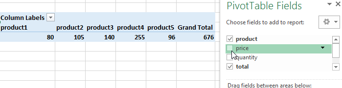
- You can remove the tick from the PRICE and tick off it next to the TOTAL PRICE. And then we get the PivotTable for the value of goods, as well as the grand total again.
Download example transpose data in Excel.
This is a rather peculiar method of partial transposition, which allows you to replace the columns in the rows (on the contrary - it does not work) and additionally learn to the total amount of the given field.

Data Visualization Charts for Interactive Report Creation in Excel.
Dashboard Templates