Autocomplete of the cells in Excel from another data table

On one of the sheets of the Excel workbook, there is the database of the business car registration data. On the second sheet is maintained the register of the delegation, where personal data of employees and cars are entered. One of the vehicles is repeatedly used by employees and each time the data enters into the register – this requires unnecessary time for the operator. It is better to automate this process. To do this, you need to create a formula, that will automatically pull up this information about the service car from the database.



Autocomplete to the cells by data in Excel

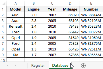
For the sake of illustration, we will schematically display the registration data base:

As it was described above, the register is on the separate Excel sheet and looks like this:

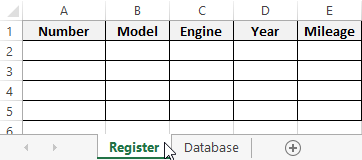
Here we implement the autocomplete Excel table. Therefore you need to note, that the names of columns headings in both tables are the same, but ones only shuffled in different order!

Let`s consider now, what you need to do after entering the registration number in the register as a value for the cell in column A, the other columns are automatically filled with the appropriate values.

How to make the autocomplete cells in Excel:

1. In the «Register» sheet you need to enter in the cell A2 any registration number from the column E on the «Database» sheet.
2. Now, in the cell B2 in the «Register» sheet, you need to enter the cell auto-complete formula in Excel:
3. You need to copy this formula to all other cells in the second row for columns C, D, E on the «Register» sheet.

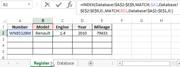
As a result, the table is automatically filled with the corresponding values of cells.



The principle of the formula for autocomplete cells

The main role in this formula is played the INDEX function. Its first argument specifies the source table that is in the car database. The second argument is the line number, that is computed using the MATCH function. This function performs to the searching in the range E2:E9 (in this case, vertically) to determine the position (in this case, the line number) in the table on the «Database» sheet for the cell, that also contains the value is entered in the «Register» sheet in A2.

The third argument for the INDEX function is the column number. It is also calculated by the MATCH formula with its other arguments. Now the MATCH function must return to the column number of the table from the «Database» sheet, that contains the name of the header corresponding to the original header of the column of the «Register» sheet. It is indicated by the reference in the first argument of the MATCH function – B$1. Therefore, this time, the value is searched only for the first line A$1:E$1 (this time horizontally) of the car registration database. The position number of the original value (this time the column number of the source table) is determined and returned as the column number for the third argument of the INDEX function.

Download the example of autocomplete cells from the another table.

Thanks to this, the formula will work even if the order of the columns will be shuffled in the register table and database. Naturally, the formula will not work, even if the column names in both tables do not match for obvious reasons.