Percent deviation formula in Excel for calculating mark-up
The concept of rejection percentage means the difference between two numeric values in percent. Let's give a concrete example: for example, one day from the warehouse were sold 120 plane tablets, and in the next day – 150 ones. The difference in sales volumes is obvious: 30 pieces more sold tablets the next day. When subtracting from the 150-th number of 120, we get a deviation, which is equal to the number +30. The question arises: what is the percentage deviation?
How to calculate the percentage deviation in Excel
The percentage of deviation is calculated by subtracting the old value from the new value, and then dividing the result by the old one. The result of calculating this formula in Excel should be displayed in the percentage format of the cell. In this example, the calculation formula is as follows (150-120) / 120 = 25%. The formula is easy to verify: 120 + 25% = 150.
Pay attantion! If we swap the old and new numbers, then we have the formula for calculating the mark-up.
Below in the picture you can see the example, how the above calculation can be represented as the Excel formula. The formula in the cell D2 calculates the percentage of deviation between the sales values for the current and last year: =(C2-B2)/B2
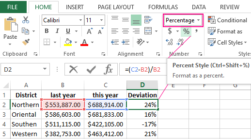
It is important to pay attention to the presence of parentheses in this formula. By default in Excel, the division operation always has the highest priority with respect to the subtraction operation. Therefore, if we do not put parentheses, the first value will be divided, and then another value will be subtracted from it. Such calculation (without parentheses) will be erroneous. Closing the first part of the calculations in the brackets formula automatically raises the priority of the subtraction operation above with respect to the division operation.
You need to enter the formula in the cell D2 correctly with brackets, and then simply copy it to the other empty cells of the D2: D5 range. To copy the formula in the fastest way, you need just to move the mouse cursor to the cursor of the keyboard cursor (to the bottom right corner), so that the mouse cursor changes from the arrow to the black cross. After that, just to make double-click with the left mouse button and Excel will automatically fill empty cells with the formula and determine the range D2: D5, which must be filled to the cell D5 and no more. This is the very convenient lifehack in Excel.
The alternative formula for calculating the percentage of deviation in Excel
In the alternative formula that calculates the relative deviation of sales values from the current year, it is immediately divisible by the sales values of the previous year, and only then the unit is removed from the result: =C2/B2-1
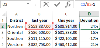
As can be seen in the picture, the calculating`s result of the alternative formula is the same as in the previous one, and therefore it`s correct. But the alternative formula is easier to write down, although it is possible for someone to read more to understand the principle of its operation. Or it is more difficult to understand what value this formula gives if it is not signed.
The only drawback of this alternative formula is that it is not possible to calculate the percentage deviation at negative numbers in the numerator or in the substitute. Even if we use the ABS function in the formula, the formula will return an error result with a negative number in the substitute.
Since in Excel by default the priority of the division operation is higher than the subtraction operation in this formula, there is no need to apply parentheses.

Data Visualization Charts for Interactive Report Creation in Excel.
Dashboard Templates