Example how to change all prices at once in Excel
In prices of Excel very often have to change prices, especially in an unstable economy.
Let's consider 2 simple and fast ways of simultaneous change of all prices with increase in the mark-up in percentage. VAT indices will be re-read automatically. And we will also learn how to calculate the mark-up in percentage terms.
How to make a mark-up on the goods in Excel?
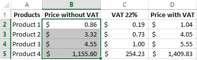
In the source table, that is a conditionally invoiced consignment note, you need to make a mark-up for all prices and VAT by 7%. How the Value Added Tax is calculated is shown in the figure:
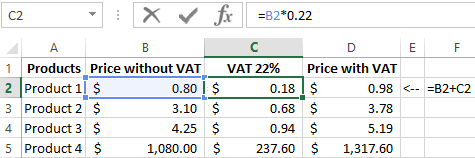
«Price with VAT» is calculated by summing up the values of «price without VAT» + «VAT». This means that it is enough for us to increase by 7% only the first column.
The method 1: price change in Excel
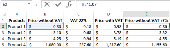
- In the column E, we calculate new prices without VAT + 7%. Enter the formula: Copy this formula to all the corresponding cells in the table in the column E. We copy also the column header from B1 to E1.
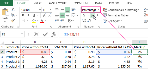
How to calculate the percentage of price increase in Excel to check the result? Very simple! In the cell F2, set the percentage format and enter the product markup formula: The markup is 7%.
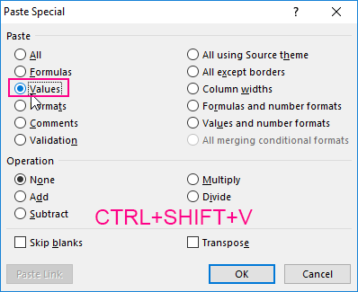
- Copy the E column and select the column B. Select the tool: «Home» – «Insert» – «Paste Special» (or press CTRL + SHIFT + V). In the window that appears, check the «value» option and click OK. Thus, the financial format of the cells has been preserved, and the values have been updated.
- We delete already unnecessary the E column. Note that thanks to the formulas, the values in the columns C and D have changed automatically.
That's all we have the price with new prices, which are increased by 7%. The columns E and F can be deleted.
The method 2 allows you to immediately change prices in the Excel column
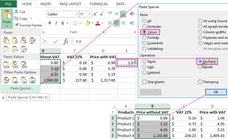
- In any cell separate from the table (for example, E2), enter a value of 1.07 and copy it.
- Select the range B2:B5. Select the «Special Paste» tool again (or press CTRL + SHIFT + V). In the appeared window, in the «Paste Special» section select the «Values» option. In the «Operations» section, select the «Multiply» option and click OK. All the numbers in the column «price without VAT» are increased by 7%.
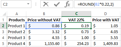
Attention! Notice, that in the cell D2 the error value is displayed: instead of 1.05 there is 1.04. These are rounding errors.
For all calculations to be correct, round numbers must be rounded up before they are summed up.
In the cell C2 add to the formula the function: =ROUND(B2*0.22,2). And you need to check: D2 = B2 + C2(1.05 = 0.86 + 0.19). Now copy the contents of the C2 to the whole range of C2:C5.
The note. Since we have only 2 terms, we do not need to round the values in the column B. Errors are already 100% will not.
Rounding errors in Excel do not surprise experienced users at all. We have already considered examples on this issue and not yet races will be considered in the following lessons.
Incorrectly rounded numbers lead to significant errors even with the simplest calculations, especially when it comes to large amounts of data. You should always keep in mind rounding errors, especially when you need to prepare an accurate report.

Data Visualization Charts for Interactive Report Creation in Excel.
Dashboard Templates