How to find an error in the Excel table according to the formula?

To save time on visual analysis of large tables in order to identify errors, it is more rationally to apply formulas for determining its location. For example, the information about the localization of the first error, that occurred relative to the rows and columns of the sheet, would be very useful.



Searching of errors in Excel by the formula

To determine of position an error location in a table with big amount of rows and columns, we recommend to take advantage of the special formula. For example we show the formula, that can easily works with large ranges of cells, within A1:Z100.

To determining to the localization of the first error on the sheet concerning of the rows, you should use to the following:

This should be executed in an array, so after entering it, you need to press to the combination of hot keys: CTRL + SHIFT + Enter. If everything is done correctly, in the formula line will be appear the curly brackets appear, as you can see in the picture.

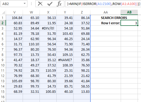
The table with large amount of data contains to errors, the first of which is in the range of the third line of the sheet 3:3.



How to get the address of the cell with an error?

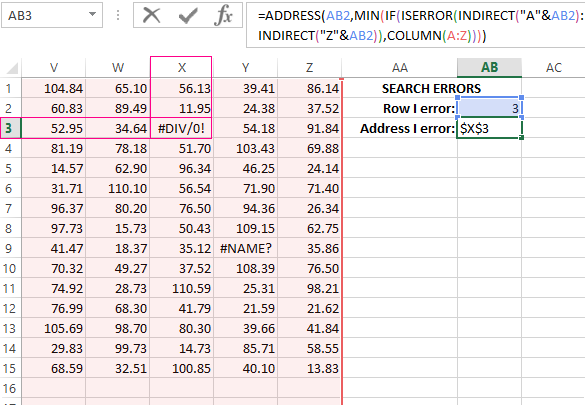
Based on the result of calculating this formula you can create to another formula that does not just define to a row or a column, but will indicate the immediate address of the error on the Excel sheet. To solve this problem below (in the cell AB 3), you need to enter to another:

This should also be executed in the array, so after entering it again, you need to press CTRL + SHIFT + Enter to confirm. The result of calculating of the local address of the cell that contains the first error in the table:

The principle of the search for error:

In the first argument of the ADDRESS function you need to specify to the line number that must be returned in the cell address, containing to the result of the action of the whole formula. The line number is defined by the previous formula and is the number 3. Therefore we only refer to the cell AB2 with the first formula. Next, using the function INDIRECT, the reference is made to the range that must be found in accordance with the location of the errors.

It is not necessary to perform to the searching on the whole table, thus loading to the processor of the computer and unnecessarily taking away the computational resources of the Excel program. We are only interested in the third line.

With helping of the ISERROR function, each of the cell in the A3:Z3 range is checked for errors. On the basis of the results obtained in an array, is created in the program memory of the logical values TRUE and FALSE. The next COLUMN function returns to the program memory to the second array of the column numbers with the numbers of elements, which corresponding to the number of columns in the range A3:Z3.

Download example find an errors in Excel

Thanks to the IF function in the first array, the logical value TRUE is replaced by the corresponding numeric value from the second array. After that, the MIN function selects the smallest numerical value of the first array, which corresponds to the number of the column, containing to the first error. Since we calculated to the row and column numbers, the calculation of the formula with the ADDRESS function is completed. It already returns by the text value for the finished cell address, which are based on the column number and the string specified in its arguments.