The Formula Bar in Excel, its settings and the purpose

Microsoft Excel is used for performing to the simple mathematical operations. The true functionality of the program is much broader.

Excel allows you to solve very complex problems, to perform unique mathematical calculations, to analyze statistical data and much more. The important element of the working field in Microsoft Excel is the formula bar. Let's try to understand the principles of its work and answer to the key questions that related to it.



What is the purpose of the Formula Bar in Excel?

The Microsoft Excel is one of the most useful programs that allows by the user to perform more than 400 mathematical operations. All of them are grouped into 9 categories:

• financial;
• date and time;
• text;
• the statistics;
• mathematical;
• arrays and links;
• the work with BD;
• brain teaser;
• the verification of values, properties and characteristics.

All these functions can be easily tracked in the cells and edited thanks to the formula bar. It displays everything that each cell contains. In the picture it is highlighted in red.

Entering the sign «=» in it, you seem to «activate» the bar and tell to the program that you are going to enter some data, formulas.



How to enter the formula in a string?

The formulas can be entered into the cells manually or using the formula bar. For writing the formula in the cell, you need to start it with the «=» sign. For example, you need to enter data into our cell A1. To do this we select it, put the «=» sign and enter the data. The line «will come to working condition» by itself. For example, we took the same cell «A1», entered the sign «=» and pressed the input for calculating to the sum of two numbers.

You can use the function wizard (fx button):

1. We to activate the required cell and go to the formula bar, find the "fx" icon and click in it.

2. It suggests immediately to choose the function =SUM(), that is necessary for the user. We select the desired option and click «OK».

3. Next in the dialog box we enter the values in the parameters of the selected function.

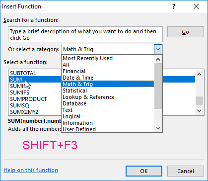
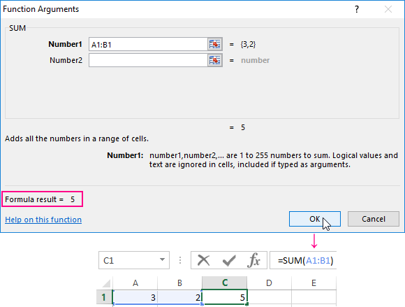
What does the Excel formula editor line contain? In practice, in this field you can:

• to enter the numbers and text from the keyboard;
• to specify the references to the ranges of cells;
• to edit the function arguments.

IMPORTANT! There is the list of typical errors that occur after an error entry, in such case the system will refuse to perform the calculation. Instead, it will give you strange values at first glance. That they were not for you cause of panic, we give their decoding.

• «#LINK!». It says, that you specified an incorrect reference to one cell or to the range of cells;
• «#NAME?». Check if you entered the correct cell address and the function name;
• «# DEL! / 0!». It says about the prohibition of division by 0. Most likely, you entered the cell with a «zero» value in the formula string;
• «#NUMBER!». It evidences, that the value of the argument of the function does not match the allowable value;
• «##########». The width of your cell is not enough to display the resulting number. You need to expand it.

All these errors are displayed in the cells, and the value in the formula line is stored after input.

What does the $ sign mean in Excel Formula Bar?

Users need to copy the formula so often, inserting it into another place of the working field. The problem is that when copying or filling out the form, the link is adjusted automatically. Therefore, you can not even «hinder» by the automatic process of the replacing the addresses of links in the copied formulas. There are relative references, that are written without the signs «$».

The $ sign is used to leave addresses for links in the formula parameters unchanged when it is copied or populated. The absolute reference is prescribed with two signs of «$»: before the letter (the column header) and in front of the figure (the title of the line). This is how the absolute link looks like: = $C$1.

The mixed link allows you to leave the value of a column or a string unchanged. If you put the «$» before the letter in the formula, then the value of the row number.

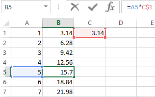
But if the formula shifts relative to the columns (horizontally), then the link will change, as it is mixed.

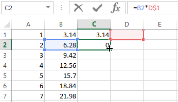
The using mixed links allows you to vary formulas and values.

The note. In order not to switch the layout every time you look for the «$» sign, you need to use the F4 key to enter the address. It serves as the link type switch. If you press it periodically, the symbol «$» is inserted automatically, making the links absolute or mixed.

The formula string was missing in Excel

How to return a string of formulas in Excel in place? The most common reason of its disappearance – is the changing of settings. Most likely, you accidentally pressed something, and this led to the disappearance of the line. To return it and continue working with documents, it is necessary to perform the following sequence of the actions:

1. To select the tab labeled «View» on the panel and click on it.
2. To check, if the tick next to the «Formula Bar» is checked. If it does not exist, we set it.

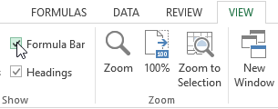
After that, the missing line in the program «returns» to the place it was assigned. In the same way, you can remove it, if necessary.

One more option. Go to the settings «File» – «Options» – «Advanced». In the right list of settings, we find the «Screen» section in the same place and check the «Show Formula Bar» option.

The Large Formula Bar

The line for entering data into the cells can be increased if you can not see a large and complex formula entirely. For this:

1. Hover your mouse over the border between the line and the column headings of the sheet so, that it changes its appearance to 2 arrows.

2. While holding to the left mouse button, move the cursor down to the required number of lines, until the content is displayed freely.

Thus, you can see and edit long functions. Also this method is useful for those cells, that contain a lot of text information.