How to raise a number to a power in Excel using the formula and operator
Often, users need to raise a number to a power. How to do it correctly with the help of "Excel"?
In this article, we will try to understand popular user questions and give instructions on how to use the system correctly. MS Office Excel allows you to perform a number of mathematical functions: from the simplest to the most complex. This universal software is designed for all occasions.
How to raise to the power of in excel?
Before searching for the required function, pay attention to the mathematical laws:
- "1" will remain "1" to any degree.
- "0" will remain "0" to any degree.
- Any number raised to zero degree equals one.
- Any value of "A" in the power of "1" will be equal to "A".
Examples in Excel:
Variant 1. Use the character "^"
The standard and easiest option is to use the "^" icon, which is obtained by pressing Shift + 6 with the English keyboard layout.
IMPORTANT!
- In order for the number to be exponentiation to the required degree, it is necessary to put the "=" sign in the cell before specifying the number you want to build.
- The degree is indicated after the sign "^".
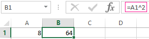
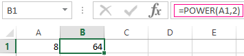
We built 8 into a "square" (that is, to the second degree) and got the result of the calculation in cell "A2".
Variant 2. Using the function
In Microsoft Office Excel there is a convenient function «POWER», which you can activate for simple and complex mathematical calculations
The function looks like this:
=POWER(Number,Degree)
ATTENTION!
- The numbers for this formula are indicated without spaces or other signs.
- The first digit is the value «number». This is the basis (that is, the figure that we are building). Microsoft Office Excel allows the introduction of any real number.
- The second figure is the value of «degree». This is an indicator in which we build the first figure.
- The values of both parameters can be less than zero ( with a "-" sign).
Formula for the exponentiation in Excel
Examples of using the =POWER() function.
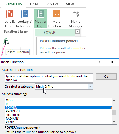
Using the function wizard:
- Start the function wizard by using the hotkey combination SHIFT + F3 or click on the button at the beginning of the formula line "fx" (insert function). From the «Or select a category:» drop-down list, select «Math & Trig», and in the bottom field «Select a function:», specify the function «POWER» we need and click OK. Or select: «FORMULAS»-«Function Library»-«Math & Trig»-«POWER».
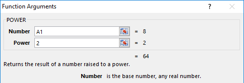
- In the dialog that appears, fill in the fields with arguments. For example, we need to exponentiate "2" to the degree of "3". Then in the first field enter "2", and in the second - "3".
- Press the "OK" button and get in the cell into which the formula was entered, the value we need. For this situation, it is "2" in the "cube", i.e. 2 * 2 * 2 = 8. The program has calculated everything correctly and has given you the result.
If you think that extra clicks are a dubious pleasure, we offer one simpler variant.
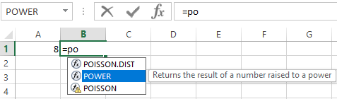
Entering the function manually:
- In the formula line we put the sign "=" and begin to enter the name of the function. Usually it is enough to write «=po…» - and the system itself will guess to offer you a useful option.
- As soon as you saw such a hint, just press the "Tab" key. Or you can continue to write, manually enter each letter. Then in parentheses, specify the required parameters: two numbers separated by a semicolon.
- After that, click on "Enter" - and in the cell the calculated value 8 appears.
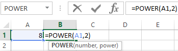
The sequence of actions is simple, and the user gets the result quickly enough. In arguments, instead of numbers, you can specify cell references.
Square root power in Excel
To extract the root using Microsoft Excel formulas, we use a slightly different, but very convenient, way of calling functions:
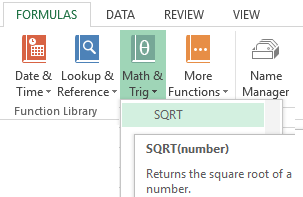
- Go to the «FORMULAS» tab. In the «Function Library» section of the toolbar, click on the «Math & Trig» tool. And from the drop-down list, select the «SQRT» option.
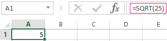
- Enter the function argument at the system request. In our case, it was necessary to find the root from "25", so we enter it into the line. After entering the number, just click on the "OK" button. In the cell, the figure obtained as a result of the mathematical calculation of the root will be reflected.
ATTENTION! If we need to know the root of the degree in Excel then we do not use the function =SQRT(). Let us recall the theory from mathematics:
"A root of the n-th degree of a is a number b whose n-th degree is equal to a", that is:
n√a = b; bn = a
"A root of n-th degree from the number a will be equal to raising to the degree of the same number a by 1/n", that is:
n√a = a1/n
From this it follows that to calculate the mathematical formula of the root in the n-th degree for example:
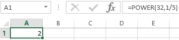
5√32 = 2
In Excel, you should write through this formula: = 32 ^ (1/5), that is: = a ^ (1 / n) - where a is a number; N-degree:

Or through this function: =POWER(32,1/5)
In the arguments of a formula and a function, you can specify cell references instead of the numbers.
How to write a number to the degree in Excel?
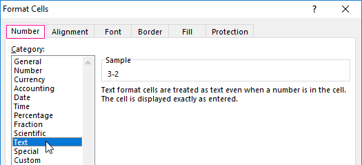
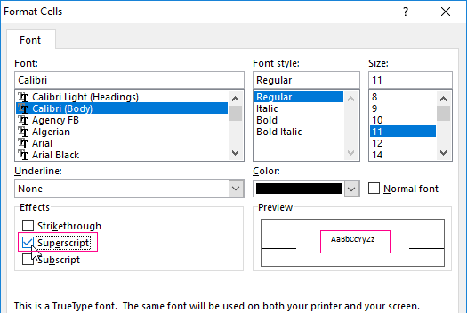
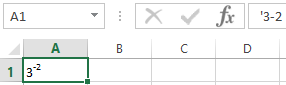
It is often important for you that the number in the degree is correctly displayed when printing and looks beautiful in the table. How to write a number to the degree in Excel? Here you need to use the Format Cells tab. In our example, we recorded "3" in the cell "A1", which should be presented to the -2 degree.
The sequence of actions is as follows:
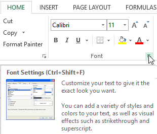
- Right click on the cell with the number and select the tab «Format Cells» from the pop-up menu. If it does not work out - find the «Format Cells» tab in the top panel or press CTRL + 1.
- In the menu that appears, select the «Number» tab and set the format for the «Text» cell. Click OK.
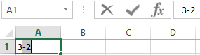
- In cell A1 enter "-2" next to "3" and select it.
- Again, we call the format of cells (for example, by pressing CTRL + 1 hot keys) and now the «Font» tab is only available for us, where we tick the «Superscript» option. And click OK.
- The result should display the following meaning:
Using Excel's features is easy and convenient. With them you save time on the implementation of mathematical calculations and the search for the necessary formulas.

Data Visualization Charts for Interactive Report Creation in Excel.
Dashboard Templates