How to remove errors in Excel cells with formulas
In case of erroneous calculations, the formulas display several types of errors instead of values. Let's consider its on practical examples in the process of formulas` work, that gave erroneous results of calculations.
Errors in Excel formula are displayed in cells
In this lesson are described to the error the values of formulas that can contain cells. Knowing the meaning of each code (for example: #VALUE!, #DIV/0!, #NUM!, # N/A!, #NAME!, #NULL!, #REF!), you will be able easily figure out how to find an error in the formula and to eliminate one.
How to remove DIV/0 in Excel?
As you can see when dividing into the cell with the empty value, the program perceives as a division by 0. The result is: #DIV/0! This can be seen with the helping of the hint.
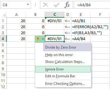
In other arithmetic calculations (multiplication, summation, subtraction), the empty cell is also zero value. Note how the error is deleted using the functions: =IFERROR(A2/B2,"") or =IF(B3,A3/B3,"") in this example.
The result of the erroneous calculation is NUM
The wrong number: #NUM! – is the error of inability to perform the calculation in the formula.
There are few practical examples:
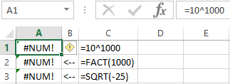
The error: #NUM! occurs, when the numeric value is too large or too small. Also, this error can occur when trying to get a root from a negative number. For example, = SQRT(-25).
- There is to much number in the cell A1(10^1000). Excel can not work with such large numbers.
- In the cell A2 – the same problem with large numbers. It would seem that 1.000 is a small number, but when you return its factorial FACT(1000), a too large numerical value is obtained, which Excel can not cope.
- In the cell A3 is the square root can not be from a negative number, and the program displayed this result with the same error.
How to remove NA in Excel?
The value is not available: #N/A! - means that the value is inaccessible to the formula:
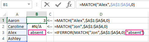
The recorded formula in B1: =MATCH («Alex», A1:A4,0) searches for the text content «Alex» in the range of the cells A1:A4. The content is found in the second cell of A3. Hence, the function returns the result 3. The second formula looks for the text content «Jon» =MATCH("Jon",$A$1:$A$4,0), then the range A1:A4 does not contain such values. Therefore, the function returns the error #N/A! (no data). The error is removed using the formula: =IFERROR(MATCH("Jon",$A$1:$A$4,0),"absent").
The error NAME in Excel
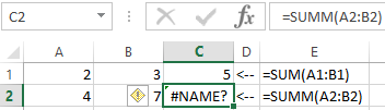
It refers to the category of errors in writing functions. There is invalid name: #NAME! – means that Excel did not recognize the text is written in the formula (it is unknown to the function SUMM name, it is written with an error). This is the result of the syntax error when writing the function name. For example:
The error NULL in Excel
The empty set: #NULL! – there are errors of the intersection operator of sets. There are such a thing as the intersection of sets in Excel. It is used to quickly obtain data from large tables by querying the intersection point of the vertical and horizontal range of cells. If the ranges do not intersect, the program displays an incorrect value – #NULL! The intersection operator of sets is the single space. It separates to the vertical and the horizontal ranges, that specified in the arguments of the function.
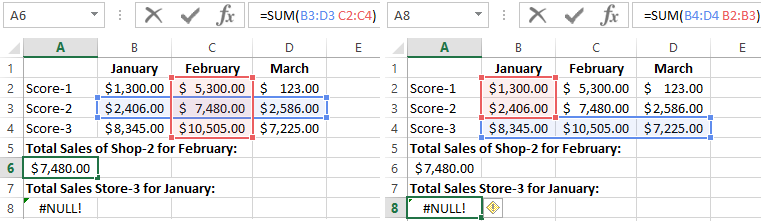
In this case, the intersection of the ranges is the cell C3 and the function displays its value.
The given arguments in the function: = SUM(B4:D4 B2:B3) – do not form the intersection. Therefore, the function gives the value with the error #NULL!
REF - the error links to Excel cells
The incorrect cell on the reference: #REF! – means that the arguments of the formula refer to the wrong address. Most often this is the non-existent cell.
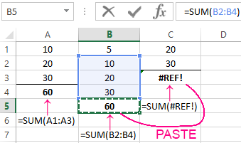
In this example, the error was occurred when the formula was copied incorrectly. There are 3 ranges of cells: A1:A3, B1:B4, C1:C2.
Under the first range into the cell A4 we need to enter the summation formula: =SUM(A1:A3). And then we copy the same formula for the second range, in the cell B5. The formula, as before, sums only 3 cells B2:B4, bypassing the value of the first B1.
When the same formula was copied to the third range, in the function cell C3, the function is returned the error #REF! Since there can be only 2 cells above the cell C3 and not 3 (as it was required by the original formula).
Note. In this case, the most convenient for each range to press the combination of the hot keys ALT + = before starting the input fast function: = SUM(). Then insert the summation function, that will be automatically determine to the number of summing cells.
The same mistake #REFERENCE! often occurs when the sheet name is incorrectly specified in the address of the three-dimensional links.
How to correct VALUE in Excel
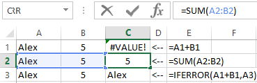
#VALUE! – is the error in the meaning. If we try to add a number and a word to Excel, as a result we can receive the #VALUE! error. There is interesting fact: if we tried to add two cells in which the value is the first number and the second is the text using the function: =SUM(), then there will be no error, and the text will take the value 0 in the calculation. For example:
The sharp ### in the Excel cell
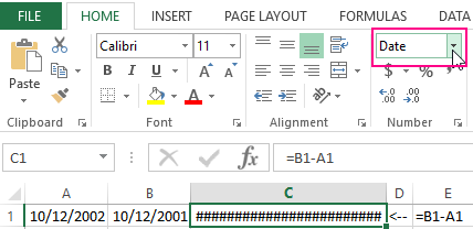
The number of sharps simbols instead of the value of the cell ###### – this value is not the error. It's just the information that the width of the column is too narrow to accommodate the correctly displayed contents of the cell. You just need to expand the column. For example, double-click the left mouse button on the border of the column headers of this cell.
So the grids (######) instead of the value of the cells can be seen with a negative date. For example, we are trying to take a new date from the old one. And as the result of the calculation, we receive the format of the cells «Date» (instead of «General») is set.
Download example remove errors in Excel.
An incorrect format of a cell can also display to the series of lattice symbols instead of values (######).

Data Visualization Charts for Interactive Report Creation in Excel.
Dashboard Templates