How to calculate discounts in Excel
For finding to the optimal value from which depends on the result of the calculation, you need to create a data table in Excel. For easy assimilation of information we give the specific example of the data table.
For major client you must make a good discount that can afford the enterprise itself. The size of the discount depends from the purchasing power of the customer. We create to the matrix of numbers for quick selection of the best combinations in terms of discounts.
Using the data table in Excel
The data table – is this simulator, which works on the principle: « and what if?» by the way of lookup values for showing all possible combinations. The simulator watches about the changing of the cell values and displays how these changes will affect to the ending result in terms of the model of the loyalty program. The data table in MS Excel allows you to quickly analyze a set of likely outcomes model. When you configure only 2 options, you can get hundreds of combinations of results and then to select to the best of them.
This tool has undeniable advantages: all results appear in the one table on one sheet.
Creating of the data table in Excel
For starters we need to build 2 models:
- The budget model company and the terms of the bonus system. To build such table you need to read the previous article: how to create a budget in Excel.
- The schema of the source data on the similarity of the «Table of Pythagoras». The string must contain a quantitative limit values for power-UPS, for example, all numbers from 100 to 500 in multiples of 50, and interest bonuses ranging from 3.0% to 10.0% of a multiple of 0.5%.
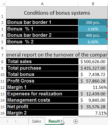
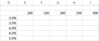
Attention! The cell (in this case D2) of the intersection of the row and column with filled values must be empty: as in the figure.
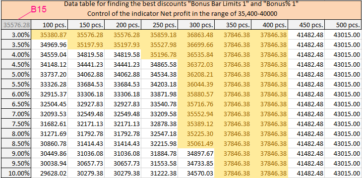
Now in the cell D2 we enter the formula is the same as for the calculation of the indicator «Margin 2»: = B15/B8 (the number format of cell is %).
Then we allocate to the range of cells D2:M17. Now for creating to the table data, you should choose to the «DATA», the section tools «Data Tools», tool «What-if Analysis» and option «Data Table».
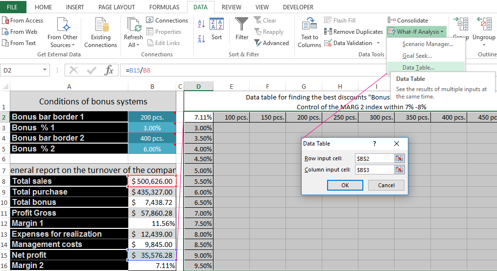
The dialog box «Data Table» will appear on the input parameters:
- The top field we fill by the absolute reference to the cell with a boundary strip of bonuses number $B$2.
- In the bottom field we refer to the value of the cell boundaries of percentage bonuses $B$3.
Attention! We expect to the optimal discounts for quantity 1 at current rates of boundary 2. For calculating discounts of quantitative discount border 2 in the boundary settings you should to show to the references on $B$4 and $B$5 are respectively.
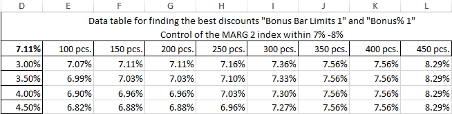
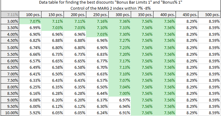
Click OK and the entire table is populated with the performance indicators «Margin 2» under appropriate conditions of bonus systems. In front of us once 135 options (all options should set to the format of cells in %).
The analysis what if in Excel data table
For the analysis using the data visualization we add to the conditional formatting:
- We allocate to the obtained results, and this is the cell range E3:M17.
- Choose to the tool: «HOME»-«Conditional Formatting»-«Highlight Cells Rules»-«Between».
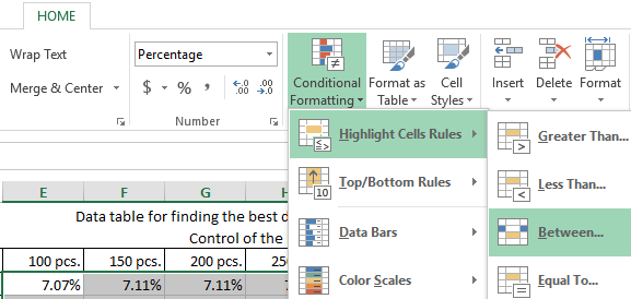
Specify to the borders from 7% to 8%, and specify to the desired format.
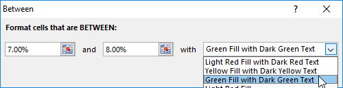
Now we can clearly see to the corridor for our profits, which we can't go out for saving to the profit in certain limits. We can easily manage by the ratio of the quantity and discount and balance between the benefit for the customer and the seller. To do this, conditional formatting allows us to make a selection of data from the Excel table according to the criteria.
Thus, we have calculated to the optimal discounts for the border 1 with the current conditions of the border 2 and its bonus.
Bonus 2 and level for border 2 in the same way expect, only don't forget to fill in the parameters correctly references $B$4 $B$5 are respectively.
The same way we can construct to the matrix for the indicator «NET Profit» and make for it to the desired conditional formatting. To mention profit with the conditional formatting we may in the range of 35 000 – 40 000.
Now you can quickly and accurately to budget the best discounts that attract customers and do not bring the damage to the enterprise.
Download enterprise budget-bonus (the sample in Excel).
When negotiating with clients the question about loyalty is raised very often about bonuses and discounts. In such cases, you can quickly build a matrix for installing of multiple borders discounts under two conditions.
Read also the beginning of this article: Budgeting of the enterprise in Excel with discounts
This is the great tool from the point of view changes in two its parameters. It quickly provides a lot of important and useful information in a clear, simple and accessible form.

Data Visualization Charts for Interactive Report Creation in Excel.
Dashboard Templates