Working with Excel array formula examples
The array of Excel functions allows you to solve complex tasks in automatically at the same time. We cannot complete the same tasks through the usual functions.
In fact, this is a group of functions that simultaneously process a group of data and immediately produce a result. Let's consider in detail work with arrays of functions in Excel.
Types of Excel functions
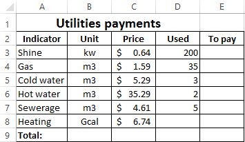
Array is a data grouped together. In this case, the group is an array of functions in Excel. Any table that we compose and fill in Excel can be called an array. Example:
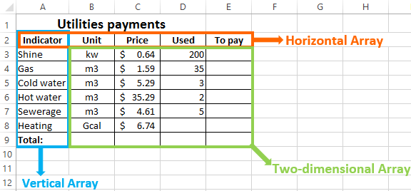
Depending on the location of the elements, the arrays are distinguished:
- One-dimensional (data is in ONE line or in ONE column);
- Two-dimensional (SEVERAL lines and columns, matrix).
One-dimensional arrays are:
- Horizontal (data in a row);
- Vertical (data in a column).
Note. Two-dimensional Excel arrays can take several sheets at once (these are hundreds and thousands of data).
Array formula allows you to process data from this array. It can return one value or result in an array (set) of values.
With the help of array formulas it is real to:
- Count the number of characters in a certain range;
- Summarize only those numbers that correspond to the given condition;
- Summarize all n values in a certain range.
When we use array formulas, Excel takes into account the range of values not as individual cells, but as a single data block.
Array formulas syntax
We use the formula of an array with a range of cells and with a separate cell. In the first case, we find the subtotals for the «To pay» "" column. In the second - the total amount of utility payments.
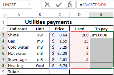
- We select the range E3: E8.
- Enter the following formula in the formula row: = C3: C8 * D3: D8.
- Press the keys simultaneously: Ctrl + Shift + Enter. The subtotals are calculated:
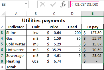
The formula after pressing Ctrl + Shift + Enter was in curly brackets. It was automatically inserted into each cell of the selected range.
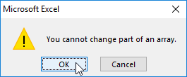
If you try to change the data in any cell in the «To pay» column, nothing happens. The formula in the array protects range values from changes. A corresponding entry appears on the screen:
Consider other examples of using the functions of an Excel array - calculate the total amount of utility payments using a single formula.
- Select the cell E9 (opposite the «Total»).
- We introduce a formula of the form:
- Press the key combination: Ctrl + Shift + Enter. Result:
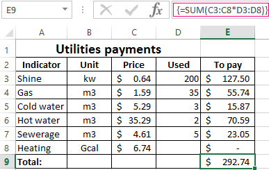
The formula of the array in this case replaced two simple formulas. This is a shortened version, which contains all the necessary information for solving a complex problem.
Arguments for a function are one-dimensional arrays. The formula looks at each of them individually, performs user-defined operations, and generates a single result.
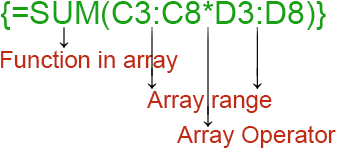
Consider the syntax:
Working functions with Excel array
Let’s guess that it is planned to increase utility payments in 10% the next month. If we introduce the usual formula for the total is =SUM((C3:C8*D3:D8)+10%), then we are unlikely to get the expected result. We need each argument to increase in 10%. For the program to understand this, we use the function as an array.
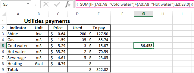
- Let's have a look how the «И» "AND" operator works in the array function. We need to find out how much we pay for the water, hot and cold. Function: The total is 86.46$.
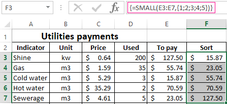
- The Sort functions in the array formula. Sort the amounts to be paid in ascending order. For the sorted data list, create a range. Let's select it (F3:F7). In the formula bar, we enter Press Ctrl + Shift + Enter.
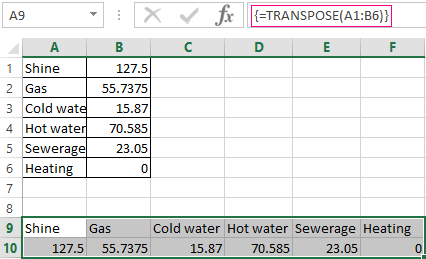
- The transported matrix. There is a special Excel function for working with two-dimensional arrays. The «ТРАНСП» function returns several values at once. It converts a horizontal matrix to a vertical matrix and vice versa. Select the range of cells where the number of rows equals to the number of columns in the table with the original data. And the number of columns equals to the number of rows in the source array. Select range A9:F10. We introduce the formula: Press Ctrl + Shift + Enter. This results in an "inverted" data set.
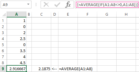
- Search for the average without taking into account zeros. If we use the standard «AVERAGE» function, we get "0" as a result. And it will be correct. Therefore, we insert an additional condition into the formula:
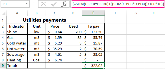
We get:
A common mistake when working with arrays of functions is NOT to press the code combination "Ctrl + Shift + Enter" (never forget this key combination). This is the most important thing to remember when processing large amounts of information. Correctly entered function performs the most complicated tasks.
