How to create a drop down menu in excel for database
A drop-down list means that one cell includes several values. When the user clicks the arrow on the right, a certain scroll appears. He can choose a specific one.
A drop-down list is a very handy Excel tool for checking the entered data. The following features of drop-down lists allow you to increase the convenience of data handling: data substitution, displaying data from another sheet or file, the presence of the search and dependency function.
Creating a drop-down list
Path: the «DATA» menu – the «Data Validation» tool – the «Settings» tab. The data type – «List».
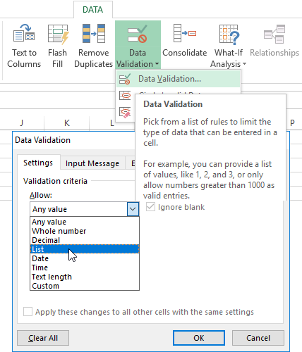
You can enter the values from which the drop-down list will consist, in different ways:
- Manually through the «Comma» in the «Source:» field.
- Enter the values in advance. Specify a range of cells with a list as a source.
- Assign a name for a range of values and enter the name in the «Source:» field.
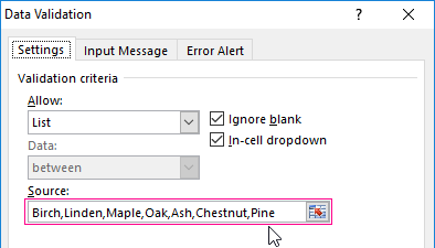
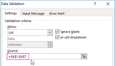
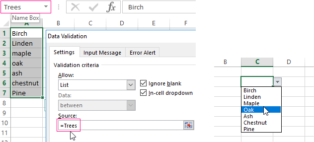
Any of the mentioned options will give the same result.
Drop-down list with data lookup in Excel
It is necessary to make a drop-down list with values from the dynamic range. If changes are made to the available range (data are added or deleted), they are automatically reflected in the drop-down list.
- Highlight the range for the drop-down list. Find the «Format As Table» tool in the main menu.
- The styles will open. Choose any of them. For solving our task, design does not matter. The presence of the header is important. In our example, the header is cell A1 with the word «Trees». That is, you need to select a table style with a header row. You’ll get the following range:
- Put the cursor on the cell where the drop-down list will be located. Open the parameters of the «Data Validation» tool (the path is described above). In the «Source:» field, write the following function:


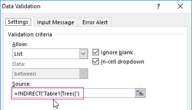
Let’s test it. Here is our table with a list on one sheet:
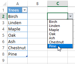
Add the new value «Spruce» to the table.
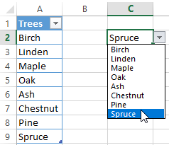
Now delete the «Birch» value.
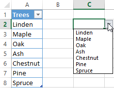
The "smart table", which easily "expands" and changes, has helped us to perform our task.
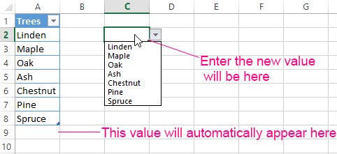
Now let's make it possible to enter new values directly into the cell with this list and have data automatically added to the range.
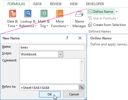
- Form a named range. Path: «FORMULAS» - «Define Name» - «New Name». Enter a unique name for the range and press OK.
- Create a drop-down list in any cell. You already know how to do this. Source – name range: =trees.
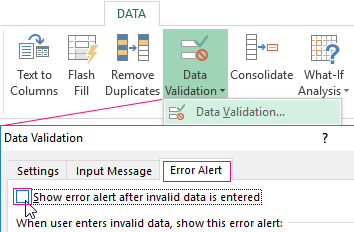
- Clear the following check boxes: «Error Alert», «Show error alert invalid data entered». If you do not do this, Excel will not allow you to enter new values.
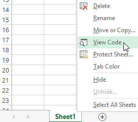
- Launch the Visual Basic Editor. To do this, right-click on the name of the sheet and go to the «View Code» tab. Alternatively, press Alt + F11 simultaneously. Copy the code (just insert your parameters).
- Save it, setting the «Excel Macro-Enabled Workbook» file type.
Private Sub Worksheet_Change(ByVal Target As Range)
Dim lReply As Long
    If Target.Cells.Count > 1 Then Exit Sub
    If Target.Address = "$C$2" Then
     If IsEmpty(Target) Then Exit Sub
       If WorksheetFunction.CountIf(Range("trees"), Target) = 0 Then
          lReply = MsgBox("Add entered name " & _
                         Target & " in the drop-down list?", vbYesNo + vbQuestion)
          If lReply = vbYes Then
              Range("trees").Cells(Range("trees").Rows.Count + 1, 1) = Target
          End If
       End If
     End If
End Sub

When you enter a new name in the empty cell of the drop-down list, the following message will appear: «Add entered name Baobab?».
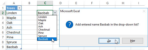
Click «OK» and one more row with the «Baobab» value will be added.
Excel drop-down list with data from another sheet / file
When the values for the drop-down list are located on another sheet or in another workbook, the standard method does not work. You can solve the problem with the help of the =INDIRECT() function: it will form the correct link to an external source of information.
- Activate the cell where we want to put the drop-down menu.
- Open the Data Validation options. In the «Source:» field, enter the following formula:
The name of the file from which the information for the list is taken is enclosed in square brackets. This file must be opened. If the book with the desired values is stored in a different folder, you need to specify the path completely.
How to create dependent drop-down lists
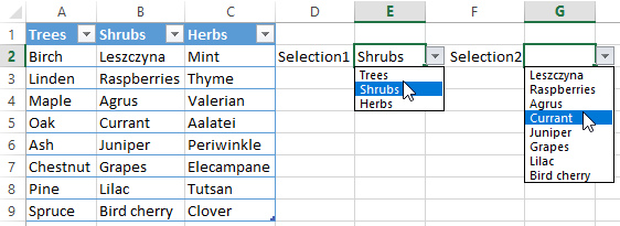
Take three named ranges:
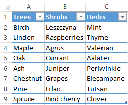
It is an indispensable prerequisite. Above you can see how to turn a normal scroll in a named range (using the «Name Manager»). Remember that the name cannot contain spaces or punctuation.

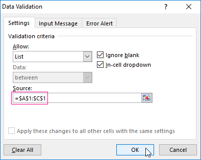
- Create the first drop-down list, which will include the names of the ranges.
- Having placed the cursor on the «Source:» field, go to the sheet and select the required cells alternately.
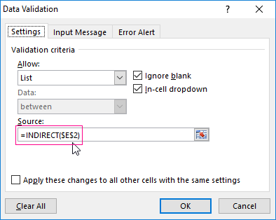
- Now create the second drop-down menu. It should reflect those words that correspond to the name chosen in the first scroll. If the «Trees», then «Linden», «Maple», etc. should correspond to it. Enter the following function: =INDIRECT(А1) in the «Source:» field. A1 is a cell with the first range.
Selecting multiple values from a drop-down list in Excel
Sometimes, you need to select several items from the drop-down list. Let's consider the ways of performing this task.
- Create a standard ComboBox using the «Data Validation» tool. Add a ready-made macro to the sheet module. The way how to do this is described above. With its help, the selected values will be added to the right of the drop-down menu.
- For the selected values to be shown from below, insert another code for processing.
- For the selected values to be displayed in the same cell separated by any punctuation mark, apply this module.
Private Sub Worksheet_Change(ByVal Target As Range)
    On Error Resume Next
    If Not Intersect(Target, Range("E2:E9")) Is Nothing And Target.Cells.Count = 1 Then
        Application.EnableEvents = False
        If Len(Target.Offset(0, 1)) = 0 Then
            Target.Offset(0, 1) = Target
        Else
            Target.End(xlToRight).Offset(0, 1) = Target
        End If
        Target.ClearContents
        Application.EnableEvents = True
    End If
End Sub
Private Sub Worksheet_Change(ByVal Target As Range)
    On Error Resume Next
    If Not Intersect(Target, Range("H2:K2")) Is Nothing And Target.Cells.Count = 1 Then
        Application.EnableEvents = False
        If Len(Target.Offset(1, 0)) = 0 Then
            Target.Offset(1, 0) = Target
        Else
            Target.End(xlDown).Offset(1, 0) = Target
        End If
        Target.ClearContents
        Application.EnableEvents = True
    End If
End Sub
Private Sub Worksheet_Change(ByVal Target As Range)
    On Error Resume Next
    If Not Intersect(Target, Range("C2:C5")) Is Nothing And Target.Cells.Count = 1 Then
        Application.EnableEvents = False
        newVal = Target
        Application.Undo
        oldval = Target
        If Len(oldval) <> 0 And oldval <> newVal Then
            Target = Target & "," & newVal
        Else
            Target = newVal
        End If
        If Len(newVal) = 0 Then Target.ClearContents
        Application.EnableEvents = True
    End If
End Sub
Do not forget to change the ranges to "your own" ones. Create scroll in the classical way. The rest of the work will be done by macros.
Searchable drop-down list in Excel
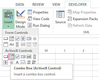
- On the «DEVELOPER» tab find the «Insert» tool – «ActiveX». Here you need the button «Combo Box (ActiveX Control)» (focus your attention on the tooltips).
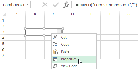
- Click on the icon – «Design Mode» becomes active. Draw a small rectangle (the place of the future scroll) with a cursor that transforms to a "cross".
- Click «Properties» to open a Combobox1 of settings.
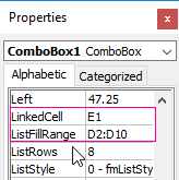
- Enter the range in the ListFillRange row (manually). The cell where the selected value will be displayed can be changed in the LinkedCell row. Changing of the font and size can be done in Font row.
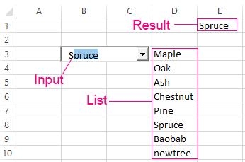
Download drop-down lists example
When you enter the first letters from the keyboard, the appropriate items are displayed. These are not all the pleasant moments of this instrument. Here you can customize the visual representation of information, specify two columns at once as a source.
