How to make a button using a macro and hyperlink in Excel
Button in Excel as a link to a cell, a tool, or a created macro, makes the work in the program much easier. Most often, it is a graphic object with an assigned macro or a hyperlink. Let’s consider how to make such a button in Microsoft Excel program.
How to make a button on the Excel sheet
The essence of the work lies in creating a graphic object and assigning a macro or hyperlink to it. Let's consider the order of actions in detail.
Ways to create a graphic object in Excel:
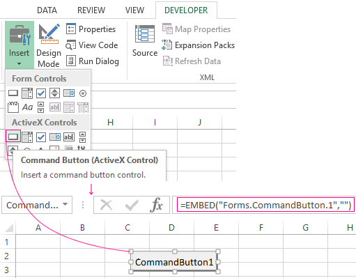
- An ActiveX control command button. Go to the «DEVELOPER» tab. Press the «Insert» ActiveX button. The menu with a set of items to insert will open. You need to select the first ActiveX element, that is depicted in in the form of a gray brick. Now draw the button of the required size using the cursor.
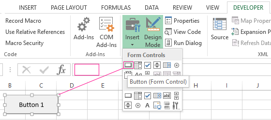
- A Form control button. Again, go to the «DEVELOPER» tab. Open the menu of the «Insert» tool. Now select the «Button (Form Control)» element from the first group (the same gray-colored brick). Then draw the button. The window for assigning a macro opens immediately: you can assign it right now or later at your option.
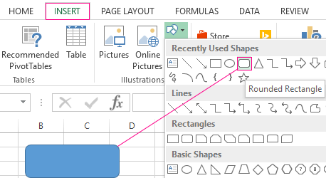
- A shape button. Go to the «INSERT» tab. In the «Recently Used Shapes» menu, select the appropriate shape. Draw this shape. You can right-click the finished shape and change its formatting.
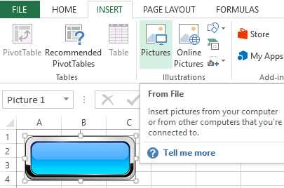
- A picture button. Go to the «INSERT» tab. In the «Illustrations» menu, select the «Pictures» tool. The options that are available on the computer will be offered to choose from.
The graphic object has been created. Now you need to make it “able to work”.
How to make a button with macro in Excel
For example, you have created a macro to perform a specific task. To run it, you need to go to the «DEVELOPER» menu every time, which is inconvenient. It is much easier to create a special button.
If you have used an ActiveX control, then:
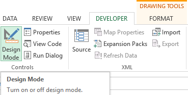
- enable the Design mode (it is on the «DEVELOPER» tab);
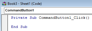
- double-click on the created button to open Visual Basic mode (ALT+F11) with the automatically created empty frame;
- enter a command between two rows to activate the macro.
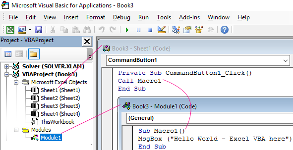
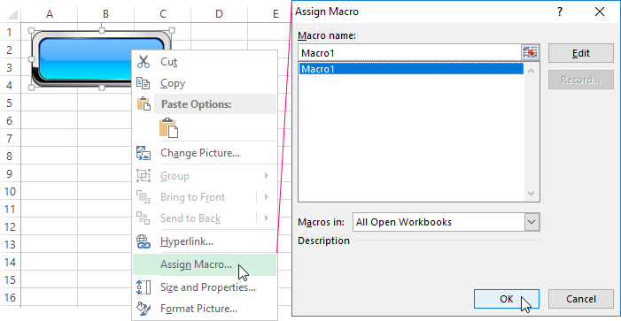
For other graphic objects, the macro is assigned in the same way. The procedure is even simpler. You need to right-click on the drawn button or picture and select the «Assign Macro» tool.
Other options of using buttons
With the help of buttons, you can not only execute created macros, but also move to a certain cell, another document, or another sheet in Excel program. Let us consider this matter in detail.
Draw a graphic object and highlight it. Find the «Hyperlink» on the «INSERT» tab.
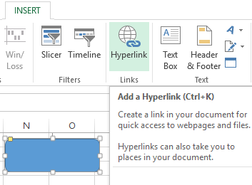
After clicking, a window will be opened. This window is intended for creating a connection between the button and a file, web page, e-mail, new document, and location in the current Excel document.
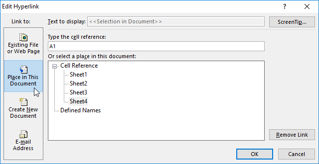
It is enough to choose the desired option and specify the path to it. This method doesn’t require writing macros and provides the user with a wide range of opportunities.
Similar tasks can be performed with the help of macros. For example, for a user to go to a certain cell (M6) when clicking the button, the following code should be written:
Sub Macro1()
Range("M6").Select
End Sub
Similarly, you can assign a macro to a chart, WordArt and SmartArt objects.
How to make the sort button for tables in Excel
For an illustrative example, create a test table as in the figure:
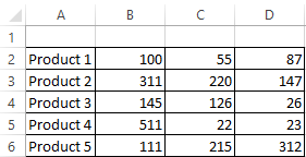
- Instead of the table column headers, add shapes that will serve as buttons for sorting by the columns of the table.
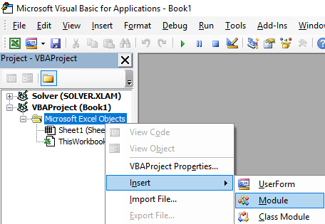
- In the Visual Basic mode (ALT + F11), insert the new module (Module1) in the Modules folder. To do this, right-click on the folder and choose Insert-Module.
- Double click on Module1 and enter the following code into it:
Note. Red text indicates different parameters for each column.
Sub Macro1()
    ActiveWorkbook.Worksheets("Sheet1").Sort.SortFields.Clear
    ActiveWorkbook.Worksheets("Sheet1").Sort.SortFields.Add Key:=Range("A2:A6"), _
        SortOn:=xlSortOnValues, Order:=xlAscending, DataOption:=xlSortNormal
    With ActiveWorkbook.Worksheets("Sheet1").Sort
        .SetRange Range("A2:D6")
        .Apply
    End With
End Sub
Sub Macro2()
    ActiveWorkbook.Worksheets("Sheet1").Sort.SortFields.Clear
    ActiveWorkbook.Worksheets("Sheet1").Sort.SortFields.Add Key:=Range("B2:B6"), _
        SortOn:=xlSortOnValues, Order:=xlDescending, DataOption:=xlSortNormal
    With ActiveWorkbook.Worksheets("Sheet1").Sort
        .SetRange Range("A2:D6")
        .Apply
    End With
End Sub
Sub Macro3()
    ActiveWorkbook.Worksheets("Sheet1").Sort.SortFields.Clear
    ActiveWorkbook.Worksheets("Sheet1").Sort.SortFields.Add Key:=Range("C2:C6"), _
        SortOn:=xlSortOnValues, Order:=xlDescending, DataOption:=xlSortNormal
    With ActiveWorkbook.Worksheets("Sheet1").Sort
        .SetRange Range("A2:D6")
        .Apply
    End With
End Sub
Sub Macro4()
    ActiveWorkbook.Worksheets("Sheet1").Sort.SortFields.Clear
    ActiveWorkbook.Worksheets("Sheet1").Sort.SortFields.Add Key:=Range("D2:D6"), _
        SortOn:=xlSortOnValues, Order:=xlDescending, DataOption:=xlSortNormal
    With ActiveWorkbook.Worksheets("Sheet1").Sort
        .SetRange Range("A2:D6")
        .Apply
    End With
End Sub - Assign to each shape its own macro: Macro1 for «NAME» Macro2 for «May», and so on.
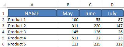
That's all, now you just need to click on the header and the table will sort the data to a particular column. For convenience, Macro1 sorts the column «NAME» in ascending order due to Order:=xlAscending parameter. All other columns have assigned macros (2,3,4) with Order:=xlDescending parameter, which sets the sort type in descending order. This is done in order to show the user in which month more goods have been sold.
Download example of the sort button
Note. Such simple macros can be created in automatic mode without programming or without writing VBA (Visual Basic for Application) code, using the «Record Macro» tool.
