CHOOSE Function in Excel: Syntax and Usage Examples
The CHOOSE function finds and returns a value from a list of arguments using an index number. It can handle up to 254 values. It has a simple syntax but quite broad capabilities. Let’s explore the best of these with practical examples.
Arguments and Syntax Features
Function syntax: =CHOOSE(index number; value 1; value 2; …).
Arguments:
- Index number – the ordinal number of the argument to be selected from the list. It can be a number from 1 to 254, a reference to a cell with a number from 1 to 254, an array, or a formula.
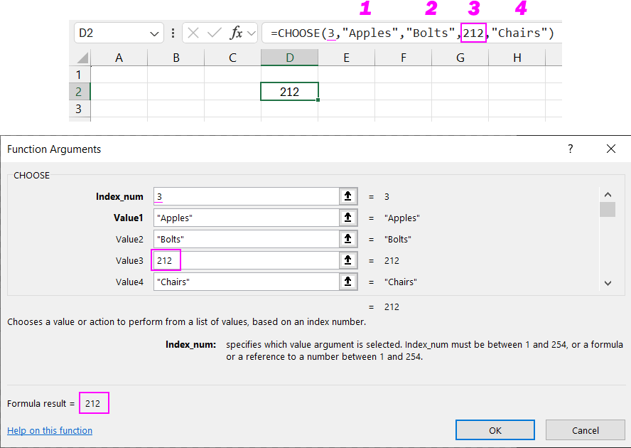
- Value 1; Value 2; … - a list of arguments from 1 to 254, from which a value or action corresponding to the index number is selected. The first value is a required argument. Subsequent ones are optional. The argument values can be numbers, cell references, names, formulas, functions, or text.
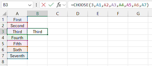
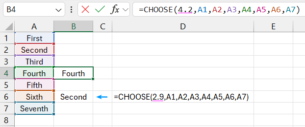
If the index number is 1, the function will return the first value in the list. If the index is 2, it will return the second value, and so on. If the list consists of specific values, the CHOOSE formula returns one of the values according to the index.
If the arguments are cell references, the function will return the references.
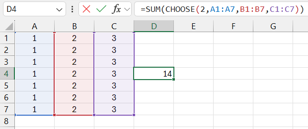
CHOOSE returns a reference to the range B1:B7. The SUM function uses this result as an argument.
Argument values can be individual values:
Function usage features:
- If the index is a fraction, the function returns the lower integer value.
- If the index is an array of values, the CHOOSE function evaluates each argument.
- If the index does not match the number of the argument in the list (less than 1 or greater than the last value), the function returns the #VALUE! error.
Examples of Using the CHOOSE Function in Excel
The CHOOSE function solves tasks related to displaying values from a list in Excel. For example, the range A2:A8 contains the week numbers from 1 to 7. You need to display the day of the week in words, such as “Monday,” “Tuesday,” “Wednesday,” “Thursday,” “Friday,” “Saturday,” and “Sunday.”
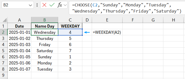
Similarly, you can display grades, scores, or seasons in words.
Now, let’s consider word declension using Excel. For example, the word "ruble": "0 rubles," "1 ruble," "2 rubles," "3 rubles," "4 rubles," "5 rubles," etc.
With the CHOOSE function, you can return a reference to a range. This allows you to perform calculations on data arrays based on user-specified criteria. Let's look at an example of calculating revenue for a user-specified store.
There is data on revenue from several retail outlets:
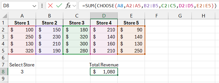
The formula calculates the revenue for the store specified by the user. In cell A8, you can change the store number – CHOOSE will return a reference to a different range for the SUM function. If you enter the number 2 in cell A8, the formula will calculate the revenue for the second store (the result of SUM for the range B2:B5).
With the CHOOSE function, you can set an argument for the SUM function to get the result of summing the first 2, 3, 4, etc. values in a range:
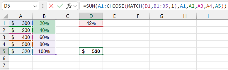
The formula sums the range A1:A2. The second part of the SUM function's range is set using the CHOOSE function. The sum range can be changed dynamically. The calculation result of the formula will look like this:
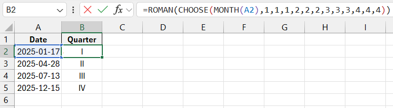
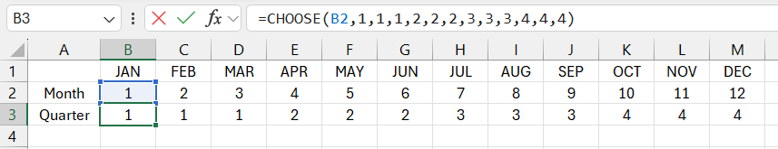
This function processes simple lists of numbers very well. Therefore, it can be used to determine the financial quarter based on the month number.
Table with month numbers and quarters:
Download examples of using the formula CHOICE in Excel 
Since the fiscal year started in January, months 1, 2, and 3 fall into the first quarter. When entering function arguments, the quarter numbers must be entered in the order they appear in the table. For some companies, the fiscal year may start in April or September, depending on the seasonality of the industry.

Data Visualization Charts for Interactive Report Creation in Excel.
Dashboard Templates