Errors in Excel Formulas when Rounding and Entering Data
Excel tries to make our work easier with auto-corrections and suggestions. When these align with our expectations, we love the program. However, when an auto-correction leads to an error, it can be quite frustrating.
One common issue arises during rounding of decimal numbers. Let’s explore why rounding errors often occur, as this operation plays a significant role in pricing and calculations. Understanding these potential errors early can help you avoid issues later on.
Errors in Rounding Decimal Numbers
How do you correctly round and sum numbers in Excel?
To illustrate, enter decimal numbers such as 1.3 and 1.4 into cells as shown in the image below, and then create a formula to sum them.
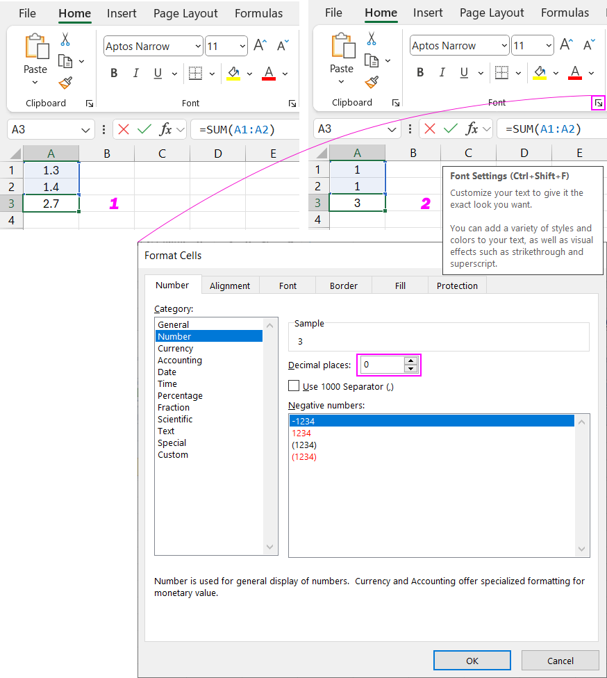
Next, highlight the numbers and the formula, then reduce the number of decimal places to round them.
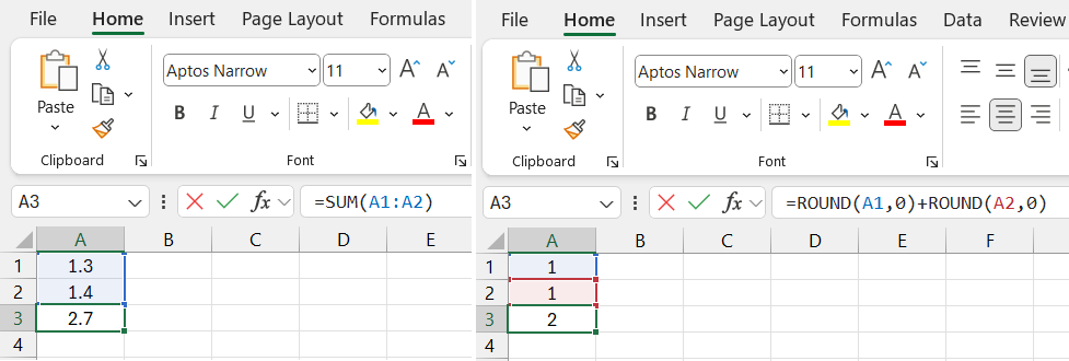
As you can see, the result might be surprising: 1+1=3. No formatting changes will fix this. To address this issue, use the ROUND function. Write the formula as: =ROUND(A1,0)+ROUND(A2,0).
Summing and Rounding Numbers in a Column
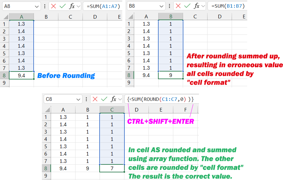
If you have a whole column of numbers, you can get accurate results quickly by using array formulas. Enter the following formula: =SUM(ROUND(A1:A7,0)). After entering the array formula, press Ctrl+Shift+Enter instead of just Enter. Excel will add curly brackets "{}" around the formula, indicating that it's an array formula. Here's an example of the result:
There's a more extreme approach, but it’s not recommended. You can force Excel to change the content of cells based on their format by going to "File" → "Options" → "Advanced" and selecting "Set precision as displayed" under the "When calculating this workbook" section. A warning will appear: "Data will be permanently changed - precision will be reduced!"
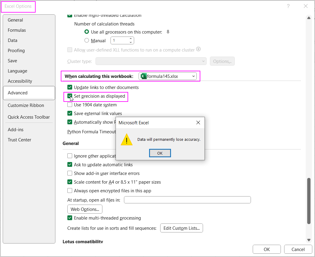
Warning!!! Once you change the number of decimal places in this way, you cannot revert to the original data. This is a one-way operation, so it's better to avoid using it. Array formulas are a safer way to handle rounding issues.
Writing TRUE or FALSE as Text in Excel
Sometimes you need Excel to treat the words "TRUE" and "FALSE" as text rather than logical values. There are two methods to achieve this:
- Prefix the text with a formatting symbol.
- Change the cell format to "Text."
Let’s implement these methods:
Task 1: In cell A1, type the word "TRUE" with a formatting symbol, like this: 'TRUE. The apostrophe (') can be typed using the English keyboard layout. Excel will hide the apostrophe and treat "TRUE" as text.
Task 2: In cell A2, change the cell format to "Text" by pressing Ctrl+1 or using the context menu. In the "Number" tab, select "Text" and click OK. Then enter the word "TRUE" in cell A2.
Task 3: For comparison, write the word "TRUE" without any changes in cell A3.
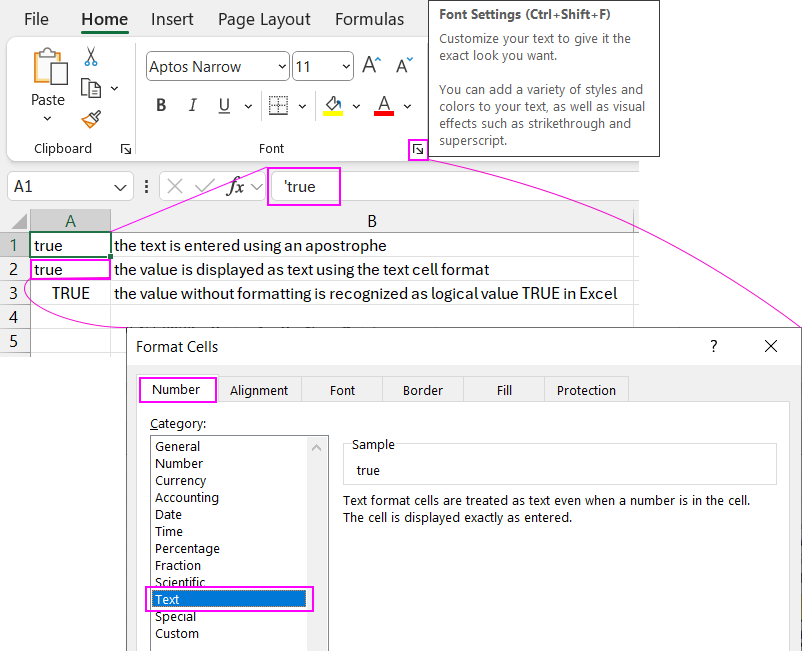
As you can see, the apostrophe is only visible in the formula bar.
Note: In cells A1 and A2, the text was not auto-corrected to uppercase because Excel interpreted it as text, not logical data.
Displaying Formulas as Text
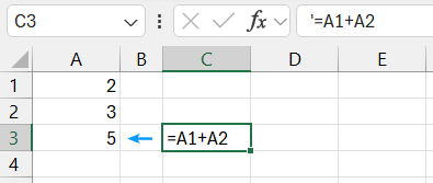
Fill the cells with data as shown in the image below:
Download examples for solving rounding and data entry issues in Excel
Normally, the combination of symbols entered in B3 would be treated as a formula and automatically calculated. But what if you want to display the text as-is, without calculating it? You can solve this using the method described earlier.
