Example Formula for Dynamic Cell Range Selection in Excel
Automatically determining the "from-to" range in the source table can be applied to automate many tasks related to dynamic value selection. Let's look at one of the simple methods for implementing this task.
How to Automatically Select Ranges for Cell Selection from a Table?
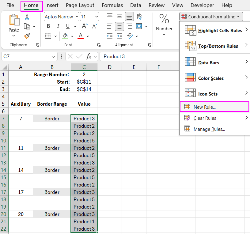
The task is as follows. In one of the columns, there are some values in different cells (in this case, the text strings "Border"). They define the start and end of sectors (ranges). These values are inserted automatically and can appear in different cells. Their sizes and the number of cells within them can also vary. For example, in the image below, data sector (range) number 2 is selected.
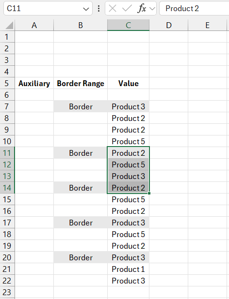
All that needs to be done now is to create an easy and quick way to select the range we're interested in (by entering the range number in one of the selection cells).
Dynamic Determination of Cell Selection Boundaries
For clarity, let's solve this task using an auxiliary column. In the first cell of the auxiliary column (A7), enter the formula:
=IF(B7="Border",ROW(),"")
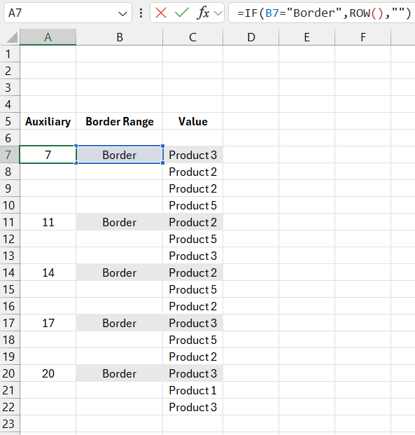
and copy it down to the remaining cells. Wherever the value "Border" is found in the adjacent column, the function returns the row number. Otherwise, it returns an empty string.
The next step is to dynamically determine the address for selecting a data range from the source list based on the selection criteria.
The changing criterion value for controlling data selection from the table will be specified in cell C1. There, we indicate the serial number of the range whose data we're interested in at the moment.
How to Get the Address of a Cell Range in Excel?
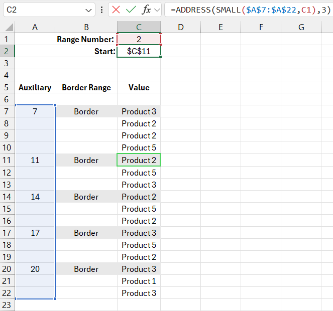
Next, we'll dynamically determine the address of the starting cell, where the range will begin. In C2, enter the following formula:
=ADDRESS(SMALL($A$7:$A$22,C1),3)
In the second argument of the SMALL function, refer to cell C1, where the serial number of the data sector (range) of interest is located. For the SMALL function, this value is the serial number of the smallest number in the auxiliary column range $A$7:$A$22 (the first argument).
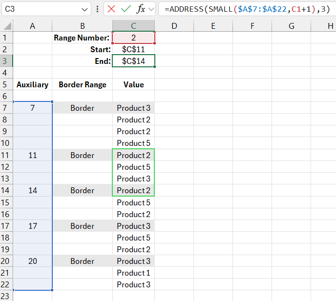
Similarly, we dynamically determine the address of the last cell, where the selection should end. To do this, enter the following formula in C3:
=ADDRESS(SMALL($A$7:$A$22,C1+1),3)
It's not hard to guess that in the second argument of the SMALL function, we add one to get the next smallest value in the auxiliary column $A$7:$A$22. It's simple and elegant - that's how magic should be!
That's practically it. Now use your imagination to apply this useful function for automatic data range selection from a table based on user conditions. For example, you can use conditional formatting.
Automatic Cell Range Highlighting Based on a Condition
We will highlight the range that corresponds to the serial number specified in the selection criteria C1.
- Select the cell range C7:C22 and choose the tool “HOME”-“Conditional Formatting”-“New Rule.”
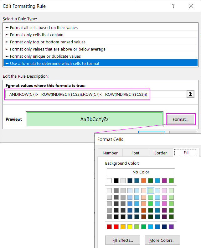
- In the window that appears, select the option “Use a formula to determine which cells to format.” Then, in the input field, enter the following formula:
- Click the Format button and choose a color to highlight the corresponding cells. For example, green.
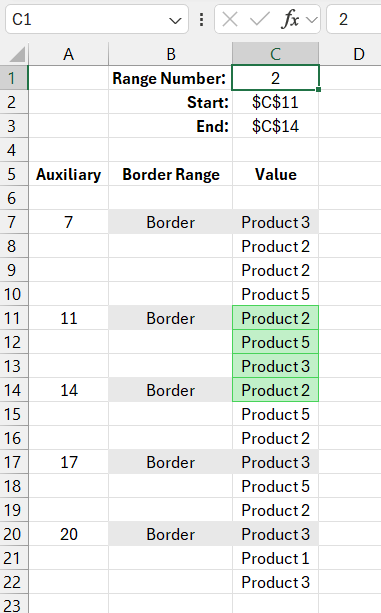
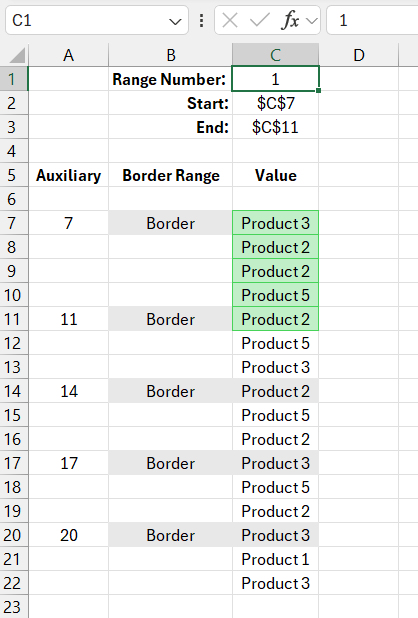
Now, let's change the selection criterion, for example, to 1. The entire first range will be automatically highlighted in green. Notice that it has one more cell than the second one, but everything works flawlessly.
Checking Input Values in Excel for Errors
Finally, you can prevent errors if an incorrect value (a number less than or equal to zero or greater than the total number of ranges) is entered as the range number you are looking for. You can do this using data validation. Go to the cell for entering the selection criteria, C1, and choose the tool: “DATA”-“Data Validation.”
The corresponding formula "ensuring safety" might look like this:
=AND($D$7>0,$D$7<COUNTIF($C$13:$C$28,"Border"))
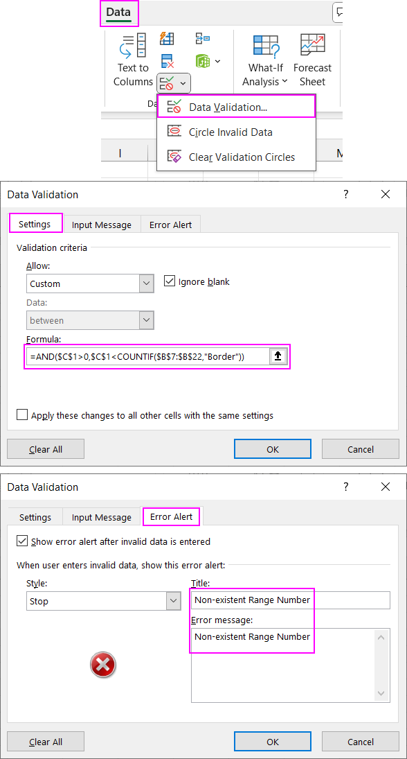
Click OK after making all the changes as shown in the image above.
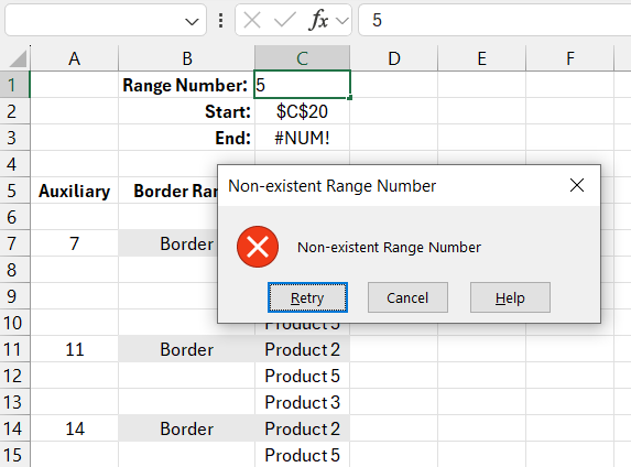
Now, if you try to enter in the selection criterion a number greater than the number of ranges within the "Borders," a warning will be displayed to the user:
Download examples of formulas for determining cell ranges in Excel 
This selection can be used in automating other various interesting tasks. Here is just a basic example of the possibilities for dynamic data selection from the source table.
