Example Formula for Highlighting Overdue Dates in Excel
In many businesses, particular attention is paid to dates that fall after a specific period has passed. With conditional formatting, you can easily create a "Past Due" report where overdue dates are highlighted.
How to Highlight Cells with Overdue Dates in Excel
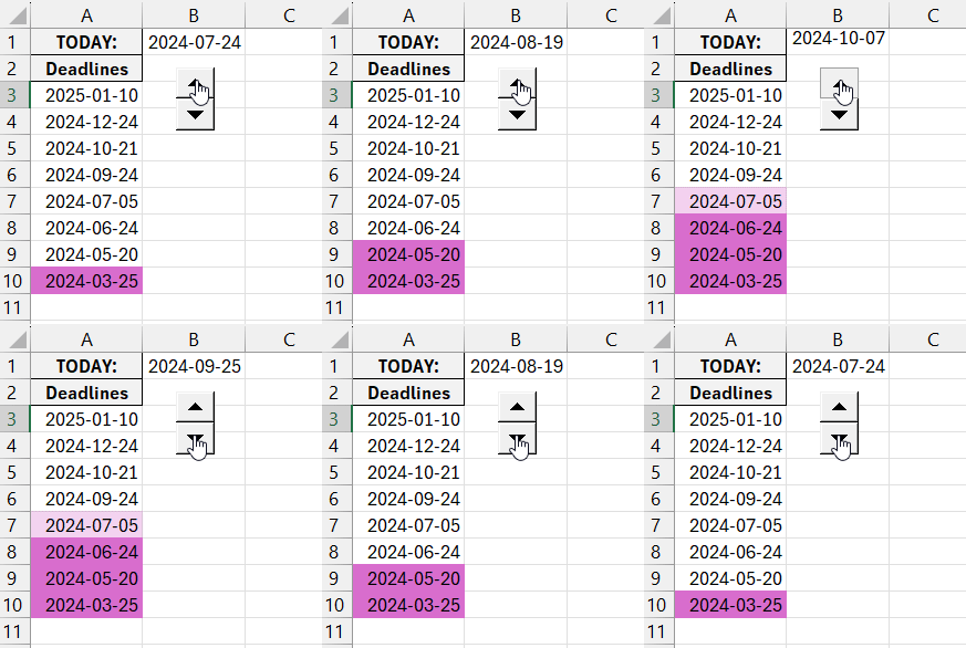
The example below shows a report where dates that are more than 90 days past the current date are highlighted with a different fill color.
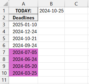
To create a similar report with automatic conditional formatting based on overdue dates, follow these steps:
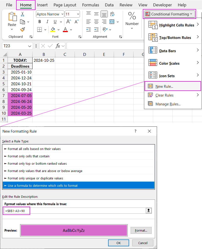
- Select the target range of cells (in this example, A3:A8) and choose the tool: "HOME" - "Conditional Formatting" - "Create Rule." This will open a window where you can input the necessary settings:
- In the window that appears, select the option "Use a formula to determine which cells to format." This allows you to create custom rules for conditional formatting using formulas. The formula should contain a logical expression and return a TRUE or FALSE value for each cell in the selected range. If TRUE, the cell will be formatted based on the predefined settings.
- In the formula input field, enter the following logical expression. This formula checks whether the date in the selected cells falls more than 90 days after today’s date. It calculates the difference between the current date (in cell B1) and the target cell (A3). If the result is greater than 90, the formatting is applied.
=$B$1-A3>90
- Click the "Format" button to open a window where you can set the desired formatting options such as fill color, font size, borders, etc. After specifying the formatting, click OK on all open windows to apply the settings and see the results.
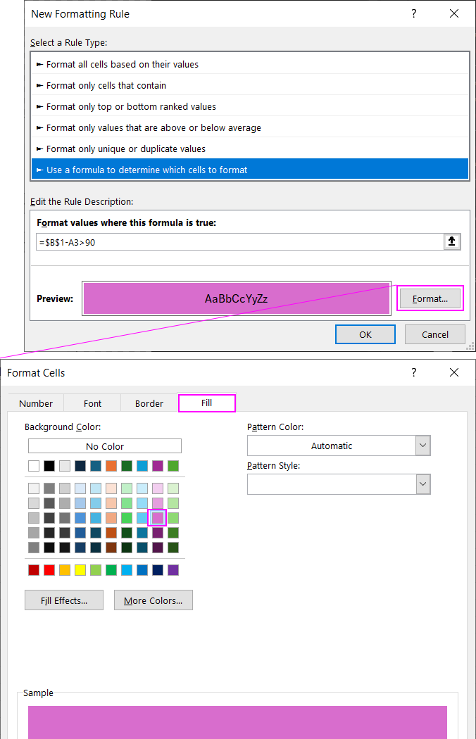
Now, whenever the current date changes, the color highlighting will automatically update based on the overdue condition set in the formula.

Download the Example Formula for Highlighting Overdue Dates in Excel 
As a result, all dates that are more than 90 days overdue are highlighted in color.
